The Current Derivative for Exponents ax is Wrong
© Miles Mathis Abstract: This is Miles Mathis' newest attempt to apply his new calculus to exponential functions. MM will show that the current derivative for exponents ax is not correct. MM will also show that the derivative for ex, though correct in some ways, is proved in a faulty manner. The proof from ln(x) is completely compromised, and MM saves the derivative of ex only by showing it is a subset of ax. This is opposite the current method, which proves ax from ex. MM will also show that the slopes of these functions are not the current values, and not the values of their derivatives (defined in a certain way). Thus MM will then show that the calculus is taught upside down. The calculus derivatives, though false, are numerically pretty accurate most of the time, but calculus is far from perfect, and that has always been known. It is known just by looking at the current manipulations, which are a jungle of ill-defined pushes and pulls; but, more importantly, it is known by the big failures of the calculus in the 20th century. MM comes to this problem from physics, and it is his belief that all or most of the point problems in QED and General Relativity are caused by the sloppy definitions and manipulations of the modern calculus. Thus MM is not trying to be contrary or revolutionary, which is in vogue today, but is trying to solve the problems that most top scientists have encountered in General Relativity and Quantum ElectroDynamics, many of which may have their root cause in faulty calculus. Those who say that Relativity is perfect must admit to a pile of Lorentz violations that now stack to the Moon, the Pioneer and Saturn anomalies, the the failure to unify GR with QED, the complete lack of a mechanism for gravity, and the solutions at zero in Black Holes. QED, which is called the most successful theory of all time, the crown jewel of physics, is a jumble of renormalization, which its inventor Feynman called hocus-pocus. QED has failed to be unified, failed to be mechanical, and failed to explain mass or charge. QED requires borrowing from the vacuum with magical incantations, requires symmetry-breaking to correct its gauge fields, and requires a ridiculous string theory to bypass reality. In A Redefinition of the Derivative and the Integral MM reinvents and reinterprets the calculus of finite differences. Opponents say it can only apply to the integers and that, having not properly generalized the derivative equation, even with regard to real numbers, that this correction and simple proof is just an anomaly or a curiosity.
MM has shown in the paper above that calculus is simply garbled and false:
The variable h can neither be zero nor go to zero. Even current mathematicians admit the first part of this. At Wikipedia, it says,
Substituting 0 for h in the difference quotient causes division by zero, so the slope of the tangent line cannot be found directly. Instead, define Q(h) to be the difference quotient as a function of h:
Q(h) is the slope of the secant line between (a, ƒ(a)) and (a + h, ƒ(a + h)). If ƒ is a continuous function, meaning that its graph is an unbroken curve with no gaps, then Q is a continuous function away from the point h = 0. If the limit limh→0Q(h) exists, meaning that there is a way of choosing a value for Q(0) which makes the graph of Q a continuous function, then the function ƒ is differentiable at the point a, and its derivative at a equals Q(0).
This is amazing, because it means that in these equations, you have to go to zero twice. First, you go to zero to find the first equation. Then, because you cannot go to zero, you create a second function you can push in the gap. You fudge your fudge. You push your push.
All of this is very ugly, as most people can see. We are told that we cannot find the tangent directly, even 300 years after Newton. Yet in the paper above MM was able to find the derivative directly and precisely straight from a table of differentials, and his generalized equation is exact and complete. It is not an estimate or an approximation, since we never go to zero or to an infinitesimal.
A common complaint is that MM does not prove the equation for all numbers, only integers. However, since all numbers are defined by integers, any extension of the basic equation is true by definition. The solution is not limited to integers, because any such proof that is proved for integers is proved for all numbers, since the number line is defined by integers. Exponential notation is defined by integers. Likewise, logarithms are defined by integers and by exponential notation, so that anything proved for integers must be proved for exponents and logarithms. There is no such thing as an exponent or integer or log that is not defined by the number line, and since the number line is defined by the integers, MM's proof is generalized automatically. All we have to do is make a simple table of differentials, using the same method MM has used for integers (as he will do again below).
To be a bit more rigorous, MM's proof in the paper above is not just a proof for integers, it is a proof of cardinal numbers and the cardinal number line. Since all derivatives are defined by the cardinal number line, a proof for the cardinal number line is a proof for all derivatives, by definition. In this way, extending the proof is just busywork. In Trig Derivatives found
without the old Calculus MM has already showed briefly how to extend his proof trig functions a few years ago, but even that did not convince his detractors. It failed to convince them because they still haven't fathomed his method. Perhaps this proof that the current derivative for exponents is false will wake them from their slumbers.
[For those who think verbal explanations are just "hand waving", MM has put a formal proof from integers to reals in a footnote*. ]
To say it again, MM has ditched the entire differential notation of Newton and Leibniz and the moderns because that notation uses the wrong differentials. In MM solution, the variable h never goes to zero because it is simply the number 1. The analog of h in MM's solution is ΔΔx, and ΔΔx is just 1. The derivative is not found at a diminishing or near-zero differential, it is found at a sub-differential which is constant and which may be defined as one. In other words, the derivative is not found at an instant, and in physical problems we can even find the time that passes and the length traveled during the derivative. In A Correction to Newton's Equation a=v2/r MM has found the time that passes during a centripetal acceleration, which is supposed to be instantaneous, proving in a specific problem that going to zero was not only unnecessary, it was physically and mathematically false.
For this reason, MM has refused to create new equations to take the place of Newton's difference quotients or to replace the equations above.They simply are not necessary. The generalized derivative equation is
and since that equation is taken straight from a table of integers, it is much preferable to show the simple table than to show a generalized difference quotient. In fact, the kind of difference quotient taught today is impossible to correct, since in the true derivation there is and can be no ratio. The derivative equation we use today, proved correctly, is not proved by pushing a ratio toward zero, it is found by simple substitution. In other words, we take this equation directly from a table of differentials section of A Redefinition of the Derivative
2x = Δx2
Then generalize it to nxn-1 = Δxn
And then define Δxn as the derivative. We can call it y' or dy/dx or whatever is convenient, but there is no ratio involved, no approach to zero, and no difference quotient. This can be seen simply by looking at the table in the paper above or at a similar table below.
Newton's difference quotient and the current ratio of changes come from analyzing curves on a graph, but MM has shown that this analysis has been faulty in many ways. It is both unnecessary and logically flawed. It is unnecessary because there is a much simpler way to derive the equation, as MM has proved by doing it; and it is flawed because Newton's method implies that we can find solutions at a point, when we cannot. The points on the graph are not defined rigorously enough, so that the solution has remained unclear for centuries. This is not a quibble, since it is precisely what causes all the point problems of QED and General Relativity.
Let me show you why there is no ratio. You can see for yourself that there is no ratio in the final equation y' = nxn-1. So where does the ratio in the difference quotient still used today come from? It comes from Newton's derivation, still taught today.
y = x2
Dividing by δx is just a trick that Newton uses to get the equation at the end. It doesn't come from any graph or table of differentials; it is just a manipulation. Dividing by δx creates the ratio of changes, and it creates the approach to zero, since δx is the h in the equations way above. The manipulation was chosen because it worked, but Newton was never able to justify it. Bishop Berkeley showed in Newton's own time that the manipulation was a fudge, and Wikipedia admits today that the manipulation is still not fully understood. Even today the equation has to be pushed with a further fudge, using the Q(h) trick above. [To read more about this, go to A Redefinition of the Derivative .]
And this brings us to one last thing to discuss before we find the derivative for exponents. The standard model of calculus now tells us that the calculus of finite differences (which MM's table is a variation of) has a margin of error relative to the regular calculus. After a long period of study, MM has been able to prove this is absolutely false. In fact, it is the opposite of the truth. It is propaganda. Or, no, it is a lie, told right to your face. What the standard model tells you, to convince you of this lie, is that the calculus of finite differences cannot find solutions at an instant or point. The calculus of finite differences can only find a solution over a defined differential, which is a length. The standard model then calls this solution a margin of error. They tell us the regular calculus can find solutions at an instant, so it must be superior.
But the defined solution of the calculus of finite differences is not a margin of error, it is simply an outcome of any math or measurement. No mathematical solution can be at a point or instant, by definition, so the failure of the calculus of finite differences to find solutions at a point is not a failure of math. It is not really a failure at all. It is a logical achievement. It is an achievement because it shows that the math has remained true to the postulates of all math and measure.
Conversely, the regular calculus, in claiming to find a solution at a point or instant, is not showing its superiority over the calculus of finite differences, it is parading a logical contradiction. It is highlighting a failure to match its own postulates and axioms. The regular calculus has claimed to be able to do something that is impossible, therefore it must be flawed.
We can see this just by looking at Wikipedia again. We are told that
the tangent line to ƒ at a gives the best linear approximation to f near a, (i.e. for small h).
Approximation, notice. Then we are told
In practice, the existence of a continuous extension of the difference quotient Q(h) to h = 0 is shown by modifying the numerator to cancel h in the denominator. This process can be long and tedious for complicated functions, and many shortcuts are commonly used to simplify the process.
Then we are shown more tricks for bettering the approximation by taking h to zero in other ways. All this must mean that it is the regular calculus that has a margin of error, and that error is NOT caused by defining all numbers as lengths or differences, as with the calculus of finite differences. It is caused by not being able to logically take the denominator of a ratio to zero. A “long and tedious process” is used to force the solution to that point or zero, but that process must be illogical and illegal, since there can be no solution at zero anyway.
This means that it is the regular calculus that has the margin of error, caused by an approximating method. The calculus of finite differences has NO ERROR, since the rate of change is precise. The number equality we take from the table of differentials is a precise number equality. The differentials equal each other exactly, with no error and no approximation. The only “imprecision” of the calculus of finite differences is that the solution must be over a defined differential, not a point. But this is not a mathematical error, it is a mathematical triumph.
What was necessary was not a lot of separate difference quotients for all the various types of functions; no, what always has been necessary is a clear proof for integers and exponents, since a clear proof for integers and exponents would supply us with methods and equations for all other functions. As Kronecker said, "God gave us the integers, all else is the work of man." Once the fundamental derivative is proved, the definition of integer and exponent will automatically give us the proof for all other numbers and functions, since all other numbers and functions are defined relative to integers. The integers are based on the number 1, and all other numbers are based on the number 1. Even e is based on the number 1, since if the number 1 loses or changes its character, e must also lose or change its character: e=2.718 only if 1=1. Logarithms may have different bases, but the number line always has a base of 1. Therefore, if we prove a derivative for the constant differential of 1, we will have proved the derivative for all numbers on the cardinal number line.
To show this once again, let us look more closely at the derivative for exponents. The generalized difference quotient for exponents currently is
dax/dx = lim (ax+h – ax)
But, as before, that is both unnecessary and false. We do not go to a limit, because h is neither zero nor approaching zero. Instead, we make a simple table of differentials.
a = 1 1,1,1,1,1,1,1,1,1,1,1,1,1
What can we tell already? Well, we can tell that the current derivative for y = ax is probably wrong. The current derivative is
dax/dx = axln(a)
But a cursory glance at the table tells us that might be wrong. We can see from the table that if a = 2, we have a rather special situation. The rate of change of the first curve y = 2x (line 2 in the table above) is 2n. The rate of that change (line 9) is 2n, and the change of that change (line 15) is also 2n. Therefore, the derivative of ax when a = 2 appears to be ax. This means that for the current derivative to be correct, the value ln(a) for a = 2 needs to be 1. But it is not. The natural log of 2 is about .693.
What MM will now do is derive the proper derivative, straight from the table. Since MM showed in the power tables of "A Redefinition of the Derivative and the Integral"
and natural log tables of "The Derivatives of the Natural Log and of 1/x are Wrong" that the derivative is actually the second rate of change of our given curve, we have to study line 15 in relation to line 2.
a = 2 2, 4, 8, 16, 32, 64, 128, 256 Then we find one line directly from the other, using the basic differential equations:
Δax = ax+1 - ax
But we are not finished. Let us compare line 17 to line 4. The first term in line 4 is 3, and the first term in line 17 is 12. To compare the rates of change, we have to mesh the two series of numbers, which means we have to multiply line 17 by 1/4. But that cannot be our general transform, since it doesn't work on lines 5 and 18, or on lines 6 and 19. The general transform is 1/(a - 1)2. Which makes our derivative
dax/dx = [1/(a - 1)2][ax+2 - 2ax+1 + ax] This means that our snap analysis of a=2 was correct. The transform reduces to 1, and so ln(a) cannot apply. This new derivative equation also gives us a good number for e. If we let x=2, the derivative equals 7.39, which is the present value of e2=7.39. Let us look at some other numbers
The slope at e, x=1 is 2.71828, which confirms the current number. However, if we calculate the slopes for other values of a, we find a large mismatch with current values:
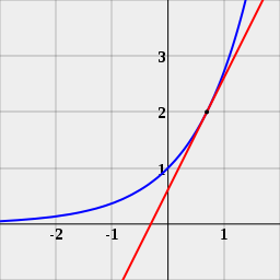
The slope at a=2, x=2 is 4, not 2.77. It appears that the derivative equation reduces to ax, which was our first guess from the table. dax/dx = ax But the slope is either not the derivative here, or we need an extra manipulation to get the slope from the derivative. The slopes just calculated for values of "a" other than e cannot be right. So let us seek the tangent and slope, damn the derivative and the rate of change of the curve. Critics have said that the calculus has long since moved past graphs and tables of differentials, but in the case of the slope and the tangent, that cannot be true. The slope and tangent are defined relative to the graph. These curve equations represent accelerations, but unless x and y are orthogonal on a graph, we will not get a curve. In real life, you can accelerate in a straight line, remember. So these accelerations were put on a graph, with x and y at right angles, specifically in order to create a curve we could analyze.
The slope is defined as Δy/Δx. Currently, the analysis takes Δx to zero to find a solution, but have shown that is both impossible and unnecessary (and it will be shown again right now, in a novel and damning way). The current method allows the calculus to find solutions at an instant and point, which is impossible. It is unnecessary, since we can find the slope without doing that. Once again, we can pull them straight from the table, without going to zero or any limit. But we will also consult a graph as we go, to see what this means there. If we let Δx=1, then we can find a slope by the first method MM has written on the graph. (4 + 2)/2 = 3. The slope at x=2 is 3. You can see that is just averaging the forward slope and the backward slope. But the historical calculus was never satisfied with that answer. Mathematicians thought, “Why not take Δx below 1, and get a more exact answer?” So they did what MM has begun to do on the graph. They looked at a smaller sub-slope, where Δx=.5. Using that smaller interval, they found a slope of 2.828. Then, by going to zero, they found a limit for that slope at 2.77. Since 2.77 is 4ln(2), they thought they had found the slope.
The problem there is that if a=2 is your base, your denominator in your slope cannot be less than 2. To see why, you have to go back to line 1 in our table above. If the base is a=1, then you get a constant differential of 1, as you see. But you want a smaller differential, so you think, “I will just use smaller values for x. I will not use 1, 2, 3. I will use .00001, .00002, .00003.” Try it, and see what happens. No matter how small you make your x's, you still get 1, 1, 1, 1, 1. Since a=2 is defined relative to a=1, what you cannot do with a=1, you cannot do with a=2.
Or, reverse this logic. Say you demand that you be able to find smaller values for a=2 in line 2. So you ignore me and just do it. Instead of 1, 2, 3, you start with .5, 1, 1.5. This gives you smaller differentials, and this allows you to take the equation 1.66 + 1.17 = 2.828 straight from the table, confirming the first step toward zero as shown on the graph. OK, but now you will have to do the same for all the values of a on the table. You say, fine. But if you do that, you will have a very strange-looking table:
a = .5 .707, .5, .354, .25, .177
Do you see the problem? You have made your Δx smaller, but it has skewed your entire solution. The rate of change of the line a=2 is not what it was before. You have changed your original curve! These two curves are not equivalent:
a = 2 2, 4, 8, 16, 32, 64, 128, 256
One curve is not double the other one, as you want it and need it to be. The first curve is the second curve squared. To say it another way: when you lowered your value for Δx, what you wanted was to put your curve under a magnifying glass. You wanted to look closer at it, moving in closer to that value of x. This is how the history of calculus is taught. This is precisely what the inventors and masters tell us they were doing. They were magnifying parts of the curve to study it. What they thought they were doing is this: when they halved their Δx, they thought they had magnified the curve by 2. In other words, in going from Δx=1 to Δx=.5, they thought they were twice as close to zero, and therefore twice as close to the limit and the answer. But it has just proved that this assumption was wrong. They were not twice as close. They were not in any proper approach to a limit. In going from Δx=1 to Δx=.5, they had not halved the curvature, they had actually gone to the square root of the curvature, so their magnification was not working like they thought it was.
Going to zero historically looked like a great idea, since it seemed to promise a more exact slope. But in going below Δx=1, the calculus has actually falsified its solution. It has found what appears to be a more exact solution only by changing its original curve. You cannot legally go below Δx=1, because that differential is what defined the curve to begin with. A smaller differential will give you a different curve and a different rate of change. What this means for our solution is that the slope at x=2 on our graph is not 4 or 2.77. It is simply 3. Our differential Δx cannot be taken below 1, due to our definitions and givens. If you go below 1, you are cheating and you are getting the wrong answer. If you desire precision in your answer, you do not take Δx to xero, your make your 1 smaller. Meaning, you set up your graph where x=1 angstrom instead of 1 meter. Our derivative method above therefore does not yield a slope. To find a slope, you use differentials from the table, but you solve in this way:
slope @ (x,y) = [y@(x + 1) - y@(x - 1)]/2 This new slope equation skews the solution for ex. If we find a slope at x=2, the slope is 8.68, not e2 = 7.39. The slope of ex is not ex. What does all this mean? It means that the calculus has been very sloppy in its math and definitions. The calculus needs to be more rigorous in defining what it wants to find from the curve. In physical situations, what the calculus wants from a curve is a velocity, but MM will show below that these curves will not give them that. Velocity is defined in a rigorous manner, and you cannot get a velocity from these curves. In pure math, the calculus claims to want to find a rate of change at a point, but since there is no such thing, we will not be able to find that either. We have just found a slope, but what does that apply to, if not to a rate of change at a point or to a velocity? Well, it applies to a rate of change at (x,y), which is the rate of change at two number values, which is a rate of change at two distances from the origin. In other words, it is a rate of change at the end of two defined intervals. As such, it is not the rate of change at a point in space. It may loosely be defined as a rate of change at a "position" in space, but that position is defined relative to other positions, and is always represented by differentials, as in distances from the origin. But why did we find different values for the slope and the derivative here? are not they the same? Not really. Again, it is a lack of rigor that has doomed us throughout history. With a=2, x=2, we found a value of 4 for the derivative and of 3 for the slope. Which is correct? Both are correct, and either can be used in math or physics. The number 4 is the change in y between x=2 and x=3. The number 3 is the average change in y midway between x=1 and x=3, and since x is changing at a constant rate, that gives us the correct value at x=2. Remember, the curvature here comes from y accelerating, not x. We put in consistent values for x, so x by itself is acting like a velocity or the pure math equivalent. No matter how big or small you make change in x, you always insert steadily increasing values, remember, as in 1, 2, 3. We never study curve equations by putting in accelerating values for x, as in 1, 4, 9, 16. So, if we define the derivative as the rate of change after a given time, rather than the rate of change at a given time, the derivative will equal the slope. In that case we can just use MM's simplified slope equation. By saying "after a given time," MM is not implying that we are calculating a total change from zero or the origin, but just reminding you that we are finding a time at specific x, and that x is telling us a distance from the origin. You will say, "If we signify a time or position 'after some time,' haven't we signified an instant or a point? is not the endpoint of any interval a point?" No, the end"point" of any interval is a position in time or space, but not an instant in time or a point in space. The position "after 6 seconds" is not at an instant, since after 6 seconds your clock does not stop running. A second is defined as an interval between ticks, but not even ticks happen at an instant. Just as you cannot measure a second with complete accuracy, you cannot have an event at a instant or point. In physics and math, there are only intervals, measured with more or less accuracy. Then you will say, "But when we actually draw a tangent to a curve on a graph, we can measure a slope more accurately than you have allowed here. Are you saying we have cheated in that also?" Yes, that is what MM is saying. For instance, let us study the graph just posted. The distance 1 is about 5/8 of an inch there. That size differential therefore defines the graph and the curve on it. You say you can tell the difference between a slope of 2.773 and 3 on that graph. First of all, accurate slopes and tangents are very difficult to find by hand, especially to curves that are curving so slightly. It is doubtful that anyone can find that accurate a slope by hand. That is why these equations were developed in the first place: you cannot do it by hand or eye. But even if you could, you would find a slope of 3 at x=2, not a slope of 2.773. You are sure you would find a slope of 2.773, but you simply trust the calculus too much. Now you say, "But you cannot be right. You are averaging two lengths of curve that are not even close to the same. The curve above that point is about twice as long as the curve below. Therefore your average has to be just a wild approximation. And yet you claim it is more accurate than the calculus which goes to zero to find precision. You must be mad!" No, you must be blind not to see that the averaging here will give us precisely the right answer without any approach to zero, since the interval above and the interval below are exactly the same size, by definition. In saying they are not, you give me the length of the curve or of y, but that is not what defines the intervals above and below. What defines them is x, and x is the same size in both places. For instance, if x were t instead, then the horizontal axis would be time. In that case, the time during the interval above and the time during the interval below would be equal. Because the intervals are equal in this way, we can average without any qualms. And that average will give us the right answer, without any approximating or error. Since x has no acceleration, all the acceleration is with y, which means we have a constant acceleration, which means we can average like this without any problem. Going to zero is not only unnecessary, it gets the wrong answer.
MM has now joined the proofs for ax and ex. MM has shown that ex is a subset of ax. MM has shown that neither are linked to ln(x), and the proofs do not rely on ln(x) or 1/x. The derivatives can be proved straight from the tables. How does the current proof find that the derivative of ax is ln(a)ax? Well, the derivative of ax is proved from the derivative of ex, and ex is proved from the derivative of ln(x). (See The Derivatives of the Natural Log and of 1/x are Wrong), so all three proofs fall with that proof. Of course, this means that the current derivative proof of ex is fudged as well. The proof starts with (given) d(lnx)/dx = 1/x. Since that is false, we know the proof is finessed. MM will show you how it is finessed:
d(lnex)/dx = d(x)/dx = 1 That is even uglier than the ln(x) proof. Concentrate on this line:
d(lnex)/dx = [d(lnu)/du] [d(ex)/dx] (Set u=ex) but work backwards. Set u=ex on its own line, like this:
d(lnex)/dx = [d(lnex)/du] [d(ex)/dx] Do you see the problem now? That cannot be equal, unless d(ex)/dx = 1. But the derivative of ex is not equal to one. Another way to look at it is that you cannot differentiate lnex with respect to u, when there is no u in the term. Or, if you substitute in the reverse way, ex=u, and create this equation d(lnex)/dx = [d(lnu)/du] [d(u)/dx] you cannot differentiate u with respect to x, when there is no x in the term. This proof is trying to rush by that manipulation, making you think that u and x have somehow been defined relative to one another in a way that allows this, when they haven't. This is just a clever juggle. If u=ex, then u and x have an exponential relationship themselves. Which means that you cannot go back and forth from dx to du so nonchalantly. Since u and x are changing at such totally different rates, differentiating with respect to u and differentiating with respect to x are not capable of substitution, not even for a moment. A final way of understanding this is that the chain rule doesn't apply to u and x when u and x are exponential to one another. This has been proved that in this very paper, showing that exponential functions are not differentiable in the common way. If they were differentiable, then the differentials would flatten. Not only do the differentials not flatten, or move toward a straight line, they do not change at all. This is the fundamental reason that the proof of the derivative of ex fails. You will say that no one is aware of that, but they should have been if they weren't. It shouldn't have required this paper to show or prove that exponents and normal variables change in fundamentally different ways. MM's table is a beautiful visualization of it, but every schoolboy knows the difference between integers and exponents.
We can see this very same error by looking at the difference quotients.
f'(a) = lim [f(a +h) – f(a)]
dax/dx = lim (ax+h – ax)
Those two equations are not analogous in form or theory. In the first equation, h is not in an exponent; but in the second equation, it is. That cannot work. And it cannot work for another fundamental reason. Look again: in the second formulation, h is exponential in the numerator, and not exponential in the denominator! So how can h be approaching zero at the same rate in both places? Exponents do not change at the same rate as normal variables. The rates are not even close, and every high school kid knows that.
This is another blunder of titanic proportions. If this basic derivative is wrong, then we must assume that the bulk of the differential equations in the standard math tables are also wrong. And if the bulk of the differential equations are wrong, then the bulk of the integrals are also wrong. As you can now see, MM's correction to the calculus requires that we recheck every single derivative and integral known to man.
How in the name of all that is holy could the entire world neglect to check the derivative against a simple list of differentials like this? Mathematicians might prefer to generalize their derivative equations without making a table every time, but you would think they would make the table the first time they calculated a basic type of derivative, like this fundamental exponential derivative, just to be sure they weren't doing their chain rules wrong or something. This is just more proof that the history of math is a cesspool of false equations.
Some will try to squirm out of this by saying that the calculus cannot be pulled from MM's tables, but if this is the case, they will have to explain to everyone how and why MM's power tables in A Redefinition of the Derivative and the Integral so successfully and easily proved the equation y' = nxn-1. It should be clear by now that MM's method of finding differentials and rates of change is both fundamental and straightforward. This method shows that the most used equation of calculus, y' = nxn-1 is correct. But it also shows that modern proofs are using a different method when finding that equation and when finding the equation dax/dx = axln(a). MM has just shown that the two methods for deriving the equations cannot be the same, since the differentials from the tables confirm the first equation and refute the second.
MM has found new and correct derivatives and slopes for ax and ex, but MM still denies that his derivative or slope is an instantaneous velocity, or any velocity. It is not an instantaneous velocity at the point x for two reasons: 1) x is not a point; x signifies a certain interval on MM's derivative curve, an interval defined by the ordered pair (x,y). Since all derivatives in the tables above are still curves, they must be curving over all intervals. The curve is not made up of either points or straight lines, so trying to assign points is impossible. Power curves can be straightened out by going to subintervals, but exponential curves cannot, as was just proved from the table. For instance, the derivative of x2 is 2x, which is a straight line. The second derivative of x3 is 6x, which is a straight line. But the derivative of ax never straightens out. Therefore, finding a velocity from a derivative with exponential functions is mathematically impossible, by the current methods. And if you do find a tangent by other more clever means, that tangent will not be the velocity at x.
In the end, it doesn't really matter one way or the other what the slope of the drawn tangent is, with exponential functions, since the slope is not the instantaneous velocity. Exponential functions are not differentiable, in that way, as MM will show below how to get an acceleration in meters and seconds from a curve equation. In other words, no real acceleration, no matter how variable, can be represented by an exponential function. Therefore we will never have to differentiate it in physics.
Something else is strange about the calculus. Notice that the derivative of a curve is a tangent, which is a straight line. But (we are told) the derivative of a velocity with respect to time is an acceleration. In one instance, we get a straight line from a curve; in the other, we get a curve from a straight line. We are told we can differentiate a line into a curve and differentiate a curve into a line. This paradox is caused by another imprecision in language. Acceleration is said to be the derivative of the velocity, but it is not. The derivative is the rate of change of the curve, and a velocity is not a curve. The derivative of any straight line is a constant, since the rate of change of any straight line is a constant. You cannot really differentiate a velocity, since there is not any variation. If you differentiate a velocity in the differential tables, you only get a line of numbers like 6, 6, 6, 6, 6. That can tell you a distance, but it cannot tell you an acceleration. Therefore, when we “differentiate” dv, we are not differentiating a velocity. This is because dv is calculus shorthand for Δv, and Δv is not a velocity; Δv is already an acceleration, by definition. An acceleration is defined as a change in velocity. When we find an acceleration “by going to zero,” what we are really finding is an “instantaneous” acceleration from an average acceleration. But, unless the acceleration is variable, the acceleration at any instant will BE the average acceleration. Instantaneous acceleration = average acceleration. This means that the equation
a = dv = lim Δv
is meaningless if the acceleration is constant. No differentiating is going on, and we are not finding a derivative. The time is not going to zero. That equation gives us exactly the same number solution as the equation a = Δv/Δt, which means that we are not going to zero or a limit. That equation is just putting the equation into calculus-speak, but no calculus is going on.
Wikipedia tells us that “the derivative of velocity with respect to time is the acceleration,” but that is simply false. In fact, it is upside down. You cannot differentiate a velocity into an acceleration, since a velocity has a constant rate of change. Conversely, if you differentiated an acceleration, you MIGHT get a velocity. Or, as MM has shown with the curve caused by the exponential function, if you differentiate an acceleration you will get another acceleration. In no case can you differentiate a straight line into a curve, or a velocity into an acceleration.
You cannot differentiate in both directions at once. You cannot differentiate a straight line (velocity) to get a curve (acceleration), and differentiate a curve to get a straight line (the tangent). One would have thought this was clear regardless.
The same applies to the equation v = dx/dt. No limit is being approached there and no derivative is being found. You cannot differentiate a distance, since there is no rate of change. That equation is just the absurd attempt to put non-calculus equations into the language of calculus. It is just a fancy and confusing way of writing v = x/t.
If we apply v = dx/dt to a curve to find an “instantaneous” velocity, then we are not finding the derivative of a distance, we are finding the derivative of the curve, and the curve is an acceleration. You are GIVEN an acceleration, and you differentiate the acceleration to find the velocity. So when Wikipedia tells us that “the derivative of the displacement of a moving body with respect to time is the velocity of the body,” the truth is on its head again. The velocity is the rate of change of the acceleration or of the curve, not of the displacement. We are differentiating the curve, not the displacement. You cannot find a derivative of the displacement.
Modern terminology is utterly reversed and topsy-turvy. Modern mathematicians appear to believe that you differentiate up from a velocity to an acceleration, when the reverse is true. The derivative is the rate of change of the curve, and the derivative flattens out the curve. When you differentiate, you go from a curve to a velocity, not from a velocity to a curve. Just look at the derivative of x2. The derivative of x2 is 2x. x2 is a curve; 2x is a straight line. The derivative straightens out the curve. And yet we are told that we differentiate a distance to find a velocity, and differentiate a velocity to find an acceleration. No wonder physics and math are completely compromised.
This means that if we differentiate a variable acceleration, we should expect to find a constant acceleration as the first derivative. With power functions, taking the derivative always straightens out the curve. Is this what we find? No. When physicists use the calculus on variable accelerations, they suddenly switch to integrals. They put v on the vertical axis and t on the horizontal axis, and use integration. This is perverse, but it is understandable. They misdefined differentiation with regard to velocity and constant acceleration, getting it upside down, so now when they come to second-degree acceleration, where they really do have to minimize their Δt in order to solve by their own method, they reverse the math. They actually integrate an acceleration to find a displacement. To do this, you have to utterly ignore the history of the calculus and the definition of “integrate.” An integration is a sum, remember, and so you integrate up from distances to velocities, and up from velocities to accelerations. You cannot integrate down. [To read more about this, see the subsection on on variable acceleration in A Redefinition of the Derivative and the Integral MM shows the modern analysis is a complete hash.]
MM promised he would show that the velocity for exponential functions cannot really be found, and he will do that now. From studying his table above, it is easy to see that no rate of change can be found, or at least no rate can be found that differs from the rate of the given equation. For a=2, the millionth derivative would have the same rate of change as the first derivative and of the curve equation itself, so differentiation, defined as straightening out the curve, is impossible. This means that the derivative listed in mathematical tables for the exponential function is just a ghost. It was a ghost even before it was shown to be false. MM's own derivative is mainly a ghost as well, though it is a correct ghost. It gives us the slope of the drawn tangent on the graph, yes, but that slope is not a velocity we can apply to a physical problem. Mathematicians have differentiated something that cannot be differentiated, and they do not seem to understand that. MM will now show you why.
Calculus was invented as a study of power series. That is fairly well understood, since we still use power series a lot, as well as Maclaurin Series and Taylor Series, and so on. MM has shown that you can also apply calculus to trig functions, simply because trig functions can be written as power functions. But many of the functions we have claimed to have differentiated are undifferentiable, and the exponential function is the prime example of this. The exponential function cannot be differentiated because differentiation is a method used on powers, not exponents. MM has shown you the fundamental reason we cannot differentiate: the table shows that the differences do not change or flatten. The physical reason we cannot differentiate is that the rate of change of the exponential equation itself is greater than any variable acceleration expressed by powers. The power x2 is a constant acceleration and the power x3 is a “variable” acceleration. All higher powers are higher accelerations. But ax, even when a=2, has a greater rate of change than any power acceleration. As a function, it is tidy only very near the origin; but at relatively low numbers for x, the function already has a gigantic slope. In fact, the slope of ax will pass the slope of any power, given a relatively short time. For this reason, we might say that, compared to the power functions, the function y=ax is infinitely variable. That is why it cannot be differentiated. As a matter of physics, the slope of ax is so near infinite, at all positive numbers except those closest to zero, that the function can be treated as a vertical line on the graph. You cannot differentiate a vertical line.
Because the function y=ax does not fail to converge in the normal ways, it is thought to be differentiable, but it is clear just from studying the tables of differentials that the function fails to converge. If it converged in the right way, the differentials would change. Since they do not, the function cannot converge and cannot be differentiated. The differentials of exponential functions do not ever flatten, they just shift.
From this, we can see that the definition of convergence for a function is incomplete. Convergence should define our ability to differentiate, which means it should define our ability to straighten out a curve by differentiation. But because the definition of convergence has been incomplete, we think we can differentiate y=ax when we cannot. We can pretend to differentiate, by finding a tangent at x, but we cannot have differentiated because the differentials themselves will not allow it.
This doesn't matter in physics because higher power accelerations there are always in the form m/sn. We do not see accelerations in the form m/nt. Time, as the independent variable in physics and life, cannot change exponentially. Time acts like a constant velocity in physics, and it is expressed to powers only to indicate multiple motions over a single interval. Therefore, we do not care whether ax can be differentiated or not, which is probably why the problems MM is uncovering have gone unnoticed.
Since velocity is defined as distance over time, and since time cannot be written as an exponential function, a real acceleration cannot be written as an exponential function. And that means that if you graph y=ax and then find a tangent at x, you cannot claim that tangent is a velocity of any kind, instantaneous or otherwise. Not only is it not the derivative of the drawn curve, it is not a velocity. It cannot be a velocity by definition of velocity and time. Modern mathematicians have simply forgotten most of the definitions of words, so they have wasted a lot of time differentiating things that cannot be differentiated and velocitizing things things that cannot be velocitized.
You will say that any straight line on a graph can be a velocity, by definition, but the problem is not in the tangent itself, it is in applying it to the curve. To call the straight line a velocity, you have to assign t to the horizontal axis. Which makes your equation y=at . That makes the relationship between distance and time exponential. But the relationship of distance and time cannot be exponential. The relationship between distance and time is always some power relationship. This is because time is operationally just a second measure of one of the distance dimensions. (See A Revaluation of Time and Velocity.) There cannot be an exponential relationship between y and t any more than there can be an exponential relationship between length and width. In space, the x-dimension and y-dimension, as dimensions, change at the same rate, so you will never find an exponential relationship between them. Since time is operationally hooked to the measure of length, the same applies to time.
This means that the calculus is not fully understood. The fact that modern mathematicians think they can integrate down from an acceleration to a distance, and think they can define the derivative up, means that history has been turned on its head. Calculus is taught upside down, nothing less. In addition, we have seen that various modern derivatives are not even correct. They are derived from compromised proofs and they get the wrong numbers. The modern calculus thinks it can take Δx to zero, not realizing that this move to a limit is changing their curve. This must mean that all of physics and math is utterly compromised. Many have wondered if they can trust newer maths like gauge maths and tensor maths and so on, and the answer is, “NO.” You cannot even trust the calculus, since physicists and mathematicians do not know how to use it. If scientists cannot do algebra and basic calculus, you can be sure they cannot do “higher” maths. Not only are higher maths completely foundationless and often false, the standard math tables of simple functions are also false (in many cases). The textbooks and standard tables cannot be trusted, even in the simplest of cases. Basic physics textbooks cover velocity and acceleration in chapter one or two, and get it wrong. This is why physics has hit a wall. It has not hit a wall because there are dimensions we do not know about or because Nature is illogical or chaotic or because the future is ruining our equations and experiments via backward causality. Physics has hit a wall because the simple math and mechanics is wrong. The basic algebra, basic calculus, and basic mechanics is full of very big holes and very big errors. That said, MM admits this paper is still not satisfactory. We know that averaging forward and backward slopes works for some curves like x2, but it is not clear that it is working here. It gets very close to the current numbers, but we need a method that can be derived right from the tables, as MM was trying to do with the differentials. MM remains convinced that going to zero is both illegal and a fudge, and that all the current proofs are finessed, but MM cannot yet see a clear way around them. .
[To read more about upside-down calculus and the basic mistakes in textbooks, see the subsection on on variable acceleration in A Redefinition of the Derivative and the Integral
*"Since it is always possible to introduce into the function f(x) a new variable whose increment is equal to one, we shall generally do so. For instance if y=f(x) and the increment of x is h, then we put x=a+hξ; from this it follows that Δξ=1; that is, ξ will increase by one if x increases by h. Therefore, starting from f(x) we find f(x) = f(a+ξh) = F(ξ) and operate on F(ξ); putting finally into the results obtained (x-a)/h instead of ξ." — Jordan, Charles. "Calculus of Finite Differences". Second Edition. New York: 1950. [Thanks to reader Diego Herrera for the reference.]
Please note that this paper is a simplification by me of a paper or papers written and copyrighted by Miles Mathis on his site. I have replaced "I" and "my" with "MM" to show that he is talking. All links within the papers, not yet simplified, are linked directly to the Miles Mathis site and will appear in another tab. (It will be clear which of these are Miles Mathis originals because they will be still contain "I" and "my".) The original papers on his site are the ultimate and correct source. All contributions to his papers and ordering of his books should be made on his site.
(This paper incorporates Miles Mathis' expon paper.)
f'(a) = lim [f(a +h) – f(a)]
h→0 h
Q(h) = lim [f(a +h) – f(a)]
h→0 h
y' = nxn-1
y + δy = (x + δx)2
δy = (x + δx)2 – x2
= 2xδx + δx2
divide by δx
δy /δx = 2x + δx
Let δx go to zero (only on the right side, of course)
δy / δx = 2x
y' = 2x
h→0 h
a = 2 2, 4, 8, 16, 32, 64, 128, 256
e = 2.718 e, 7.389, 20.086, 54.6, 148.4, 403.4, 1097
a = 3 3, 9, 27, 81, 243, 729, 2187, 6561
a = 4 4, 16, 64, 256, 1024, 4096
a = 5 5, 25, 125, 625, 3125, 15625
a = 6 6, 36, 216, 1296, 7776, 46656, 279936
Δa1 0
Δa2 2, 4, 8, 16, 32, 64, 128, 256
Δe 4.67, 12.7, 34.5, 93.8, 255, 693.6
Δa3 6, 18, 54, 162, 486, 1458, 4374
Δa4 12, 48, 192, 768, 3072, 12288
Δa5 20, 100, 500, 2500, 12500
Δa6 30, 180, 1080, 6480, 38880
ΔΔa2 2, 4, 8, 16, 32, 64, 128, 256
ΔΔe 8.03, 21.8, 59.3, 161.2, 438.6
ΔΔa3 12, 36, 108, 324, 972, 2916
ΔΔa4 36, 144, 576, 2304
ΔΔa5 80, 400, 2000, 10000
ΔΔa6 150, 900, 5400, 32400
ΔΔΔe 13.77, 37.5, 101.9, 277.4
ΔΔΔa3 24, 72, 216, 648
ΔΔΔa4 108, 432, 1728
ΔΔΔa5 320, 1600, 8000
ΔΔΔa6 750, 4500, 27000
ΔΔa2 2, 4, 8, 16, 32, 64, 128, 256
Δax+1 = ax+2 - ax+1
ΔΔax = [ax+2 - ax+1] - [ax+1 - ax]
ΔΔax = ax+2 - 2ax+1 + ax
The slope at e, x=2 is 7.393, which confirms the current number.
The slope at e, x=3 is 20.086, which confirms the current number.
The slope at a=3, x=2 is 9, not 9.9.
The slope at a=4, x=4 is 256, not 355.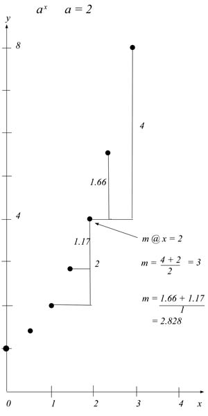
a = 1 1,1,1,1,1,1,1,1,1,1,1,1,1
a = 2 1.41, 2, 2.83, 4, 5.66, 8, 11.3, 16
a = 3 1.73, 3, 5.2, 9, 15.6, 27, 46.8
a = 2 1.41, 2, 2.83, 4, 5.66, 8, 11.3, 16
d(lnex)/dx = [d(lnu)/du] [d(ex)/dx] (Set u=ex)
= (1/u) d(ex)/dx = [1/ex] [d(ex)/dx] = 1 (equation 1)
d(ex)/dx = ex
h→0 h
h→0 h
dt t→0 Δt
Conclusion
To see other failed derivatives, you may go to The Derivatives of the Natural Log and of 1/x are Wrong where it will be shown that both derivatives are false.]