A Redefinition of the Derivative and the Integral
why
the calculus works and why it doesn't
| Please note that this paper is a simplification by me of a paper or papers written and copyrighted by Miles Mathis on his site. I have replaced "I" and "my" with "MM" to show that he is talking. All links within the papers, not yet simplified, are linked directly to the Miles Mathis site and will appear in another tab. (It will be clear which of these are Miles Mathis originals because they will be still contain "I" and "my".) The original papers on his site are the ultimate and correct source. All contributions to his papers and ordering of his books should be made on his site. (This paper incorporates the last part of Miles Mathis' calcsimp paper, are paper, power paper, calculus flaw paper and varacc paper). |
First draft begun December 2002. First finished draft May 2003 (in my files). That draft submitted to American Mathematical Society August 2003. This is the extended draft of 2004, updated several times since then

Newton Leibniz Cauchy
ObjectivesTo prove:
Index
|
Preface - Calculus Simplified
This is from the paper calcsimp, 2006
The long paper which follows this preface which also included a section on the point which was split out into a separate paper: A Physical Point has No Dimensions tackles a large number of problems that have accumulated over hundreds of years and is therefore quite intimidating. Since the wrong calculus is taught in school, the reader may wonder why it is necessary to have the subject redefined, especially since it already scary.
For this reason this shorter and simplified preface is necessary. What Miles Mathis plans to do here is try to sell his idea to a hypothetical reader, a reader who is just entering first-semester calculus. MM will explain to him or her why his explanation is necessary, why it is better, and why he or she should prefer to take a course based on his explanation rather than a course based on current theory. In doing this, it will be shown that current notation and the current method of teaching calculus is a gigantic mess. In a hundred years, all educated people will look back and wonder how calculus could exist, and be taught, in such a confusing manner. They will wonder how such basic math, so easily understood, could have remained in a halfway state for so many centuries. The current notation and derivation for the equations of calculus will look to them like the leeches that doctors used to put on patients, as an all-round cure, or like the holes they drilled in the head to cure headache. Many students have felt that learning calculus is like having holes drilled in their heads, and in that they were right to feel that way.
What some of you students have no doubt already felt is that the further along in math you get, the more math starts to seem like a trick. When you first start out, math is pretty easy, since it makes sense. You do not just learn an equation. No, you learn an equation and you learn why the equation makes sense. You do not just acquire a fact, you acquire understanding. For example, when you learn addition, you do not just learn how to use a plus sign. You also learn why the sign works. You are shown the two apples and the one apple, and then you put them together to get three apples. You see the three apples and you go, “Aha, now I see!” Addition makes sense to you. It does not just work. You fully understand why it works.
Geometry is also understood by most students, since geometry is a physical math. You have pictures you can look at and line segments you can measure and so on, so it never feels like some kind of magic. If your trig teacher was a good teacher, you may have felt this way about trig as well. The sine and cosine stuff seems a bit abstract at first, but sooner or later, by looking at triangles and circles, it may dawn on you that everything makes absolute sense.
Algebra is the next step, and many people get lost there. But if you can get your head around the idea of a variable, you are halfway home.
But when we get to calculus, everyone gets swamped. Notice that MM did not say, “almost everyone.” No, he said everyone. Even the biggest nerd with the thickest glasses who gets A’s on every paper is completely confused. Those who do well in their first calculus courses are the ones that just memorize the equations and do not ask any questions.
One reason for this is that with calculus you will be given some new signs, and these signs will not really make sense in the old ways. You will be given an arrow pointing at zero, and this little arrow and zero will be underneath variables or next to big squiggly lines. This arrow and zero are supposed to mean, “let the variable or function approach zero,” but your teacher probably will not have time to really make you understand what a function is or why anyone wanted it to approach zero in the first place. Your teacher would answer such a question by saying, “Well, we just let it go toward zero and then see what happens. What happens is that we get a solution. We want a solution, do not we? If going to zero gives us a solution, then we are done. You cannot ask questions in math beyond that.”
Well, if you teacher says that to you, you can tell your teacher does not have a clue either. Math is not just memorizing equations, it is understanding equations. All math, no matter how difficult, is capable of being understood in the same way that 2+2=4 can be understood; and if your teacher cannot explain it to you, then he or she does not understand it.
What is happening with calculus is that you are taking your first step into a new kind of math and science. It is a kind of faith-based math. Almost everything you will learn from now on is math of this sort. You will not have time to understand it, therefore you must accept it and move on. Unless you plan to become a professor of the history of math, you will not have time to get to the roots of the thing and really make sense of it in your head.
No one understands or ever understood calculus, not Einstein, not Cauchy, not Cantor, not Russell, not Bohr, not Feynman, no one. Not even Leibniz or Newton understood it. That is a big statement, but MM will prove it here, not with philosophy, but by a simple 'magic' table. Once you see the proof you will know that no understood it because, if they did, they would have corrected it like MM is about to.
It is clear that math after calculus is faith-based. Just listen a quote of Richard Feynman, who is probably the most famous physicist after Einstein, having got a lot of attention in the second half of the 20th century as one of the fathers of Quantum Electrodynamics. One of his most quoted quotes is, “Shut up and calculate!” Meaning, “Don’t ask questions. Don’t try to understand it. Accept that the equation works and memorize it. The equation works because it matches experiment. There is no understanding beyond that.”
All of QED is based on this same idea, which started with Heisenberg and Bohr back in the early 1900’s. “The physics and math are not understandable, in the normal way, so do not ask stupid questions like that any more.” This last sentence is basically the short form of what is called the Copenhagen Interpretation of quantum dynamics. The Copenhagen Interpretation applies to just about everything now, not just QED. It also applies to Relativity, in which the paradoxes must simply be accepted, whether they make sense or not. And you might say that it also applies to calculus. Historically, your professors have accepted the Copenhagen Interpretation of calculus, and this interpretation states that students’ questions cannot be answered.
You will be taught to understand calculus like your teacher understands it, and if your teacher is very smart he understands it like Newton understood it. He will have memorized Newton’s or Cauchy’s derivation and will be able to put it on the blackboard for you. But this derivation will not make sense like 2+2=4 makes sense, and so you will still be confused. If you continue to ask questions, you will be read the Copenhagen Interpretation, or some variation of it. You will be told to "shut up and calculate."
In the first semester of calculus you will learn differential calculus. The amazing thing is that you will probably make it to the end of the semester without ever being told what a differential is. Most mathematicians learn that differential calculus is about solving certain sorts of problems using a derivative, and later courses called “differential equations” are about solving more difficult problems in the same basic way. However, most never think about what a differential is, outside of calculus.
MM did not ever think about what a differential was until later, and he is not alone. This is clear because when MM tells people that his new calculus is based on a constant differential instead of a diminishing differential, they look at him like he just started speaking Japanese with a Dutch accent. For them, a differential is a calculus term, and in calculus the differentials are always getting smaller. They cannot imagine what a constant differential is.
A differential is one number subtracted from another number: (2-1) is a differential. So is (x-y). A “differential” is just a fancier term for a “difference”. A differential is written as two terms and a minus sign, but as a whole, a differential stands for one number. The differential (2-1) is obviously just 1, for example. So you can see that a differential is a useful expansion. It is one number written in a longer form. You can write any number as a differential. The number five can be written as (8-3), or in a multitude of other ways.
We may want to write a single number as a differential because it allows us to define that differential as some useful physical parameter. For instance, a differential is most often a length. Say you have a ruler. Go to the 2-inch mark. Now go to the 1-inch mark. What is the difference between the two marks? It is one inch, which is a length. (2-1) may be a length. (x-y) may also be a length. In pure math, we have no lengths, of course, but in math applied to physics, a differential is very often a length.
The problem is that modern mathematicians do not like to teach you math by drawing you pictures. They do not like to help you understand concepts by having you imagine rulers or lengths or other physical things. They want you to get used to the idea of math as completely pure. They tell you that it is for your own good. They make you feel like physical ideas are equivalent to pacifiers: you must grow up and get rid of them. But the real reason is that, starting with calculus, they can no longer draw you meaningful pictures. They are not able to make you understand, so they tell you to shut up and calculate.
It is kind of like the wave/particle duality, another famous concept you have probably already heard of. Light is supposed to act like a particle sometimes and like a wave at other times. No one has been able to draw a picture of light that makes sense of this, so we are told that it cannot be done. But in another one of his papers MM has drawn a picture of light that makes sense of this, and in this paper MM will show you a pretty little graph that makes perfect sense of the calculus. You will be able to look at the graph with your own eyes and you will see where the numbers are coming from, and you will say, “Aha, I understand. That was easy!” (See The Probability Wave of QM is not reality.)
There is basically only one equation that you learn in your first semester of calculus. All the other equations are just variations and expansions of the one equation. This one equation is also the basic equation of what you will learn next semester in integral calculus. All you have to do is turn it upside down, in a way. This equation is:
| y’ = nxn-1 |
This is the magic equation. What you will not be told is that this magic equation was not invented by either Newton or Leibniz. All they did is invent two similar derivations of it. Both of them knew the equation worked, and they wanted to put a foundation under it. They wanted to understand where it came from and why it worked,but they failed and everyone else since has failed. The reason they failed is that the equation was used historically to find tangents to curves, and everyone all the way back to the ancient Greeks had tried to solve this problem by using a magnifying glass.
What is meant by this is that for millennia, the accepted way to approach the problem and the math was to try to straighten out the curve at a point. If you could straighten out the curve at that point you would have the tangent at that point. The ancient Greeks had the novel idea of looking at smaller and smaller segments of the curve, closer and closer to the point in question. The smaller the segment, the less it curved. Rather than use a real curve and a real magnifying glass, the Greeks just imagined the segment shrinking down. This is where we come to the diminishing differential. Remember that MM said the differential was a length. Well, the Greeks assigned that differential to the length of the segment, and then imagined it getting smaller and smaller.
Two thousand years later, nothing had changed. Newton and Leibniz were still thinking the same way. Instead of saying the segment was “getting smaller” they said it was “approaching zero”. That is why we now use the little arrow and the zero. Newton even made tables, kind of like MM will make below. He made tables of diminishing differentials and was able to pull the magic equation from these tables.
The problem is that he and everyone else has used the wrong tables. You can pull the magic equation from a huge number of possible tables, and in each case the equation will be true and in each case the table will “prove” or support the equation. But in only one table will it be clear why the equation is true. Only one table will be simple enough and direct enough to show a 16-year-old where the magic equation comes from. Only one table will cause everyone to gasp and say, “Aha, now I understand.”
Newton and Leibniz never discovered that table, and no one since has discovered it. All their tables were too complex by far. Their tables required you to make very complex operations on the numbers or variables or functions. In fact, these operations were so complex that even Newton and Leibniz got lost in them. As will be shown after unveiling the table, Newton and Leibniz were forced to perform operations on their variables that were actually false.
Getting the magic equation from a table of diminishing differentials is so complex and difficult that no one has ever been able to do it without making a hash of it. It can be done, but it is not worth doing. If you can pull the magic equation from a simple table of integers, why try to pull it from a complex table of functions with strange and confusing scripts? Why teach calculus as a big hazy mystery, invoking infinite series or approaches to 0’s or infinitesimals, when you can teach it at a level that is no more complex than 1+1=2?
So here is the lesson that will teach you differential calculus in one day, in one paper. If you have reached this level of math, the only thing that should look strange to you in the magic equation is the y’. You know what an exponent is, and you should know that you can write an exponent as (n-1) if you want to. That is just an expansion of a single number into a differential, as was taught above. If n=2, for instance, then the exponent just equals 1, in that case. Beyond that, “n” is just another variable. It could be “z” or “a” or anything else. That variable just generalizes the equation for us, so that it applies to all possible exponents.
All that is just simple algebra. But you do not normally have primed variables in high school algebra. What does the prime signify? That prime is telling you that y is a different sort of variable than x. When you apply this magic equation to physics, x is usually a distance and y is a velocity. A variable could also be an acceleration, or it could be a point, or it could be just about anything. But we need a way to remind ourselves that some variables are one kind of parameter and some variables are another. So we use primes or double primes and so on.
This is important, because it means that mathematically, a velocity is not a distance, and an acceleration is not a velocity. They have to be kept separate. A calculus equation takes you from one sort of variable to another sort. You cannot have a distance on both sides of the magic equation, or a velocity on both sides. If x is a distance, y’ cannot be a distance, too.
Some people will try to convince you later that calculus can be completely divorced from physics, or from the real world. They will stress that calculus is pure math, and that you do not need to think of distances or velocities or physical parameters. But if this were true, we would not need to keep our variables separate. We would not need to keep track of primed variables, or later double-primed variables and so on.
Variables in calculus do not just stand for numbers, they stand for different sorts of numbers, as you see. In pure math, there are not different sorts of numbers, beyond ordinal and cardinal, or rational and irrational, or things like that. In pure math, a counting integer is a counting integer and that is all there is to it. But in calculus, our variables are counting different things and we have to keep track of this. That is what the primes are for.
What, you may ask, is the difference between a length and a velocity? You can probably answer that without the calculus, and probably without outside help. To measure a length you do not need a watch. To measure velocity, you do. Velocity has a “t” in the denominator, which makes it a rate of change. A rate is just a ratio, and a ratio is just one number over another number, with a slash in between. Basically, you hold one variable steady and see how the other variable changes relative to it. With velocity, you hold time steady (all the ticks are the same length) and see how distance changes during that time. You put the variable you know more about (it is steady) in the denominator and the variable you are seeking information about (you are measuring it) in the numerator. Or, you put the defined variable in the denominator (time is defined as steady) and the undefined variable in the numerator (distance is not known until it is measured).
All this can also be applied to velocity and acceleration. The magic equation can be applied to velocity and acceleration, too. If x is a velocity, then y’ is an acceleration. This is because acceleration is the rate of change of the velocity. Acceleration is v/t. So you can see that y’ is always the rate of change of x. Or, y’ is always x/t. This is another reason that calculus cannot really be divorced completely from physics. Time is a physical thing. A pure mathematician can say, “Well, we can say that y’ is always x/z, where z is not time but just a pure variable.” But in that case, x/z is still a rate of change. You can refuse to call “z” a time variable, but you still have the concept of change. A pure number changing still implies time passing, since nothing can change without time passing. Mathematicians want “change” without “time”, but change is time. If a mathematician can imagine or propose change without time, then he is cleverer than the gods by half, since he has just separated a word from its definition. (See A Revaluation of Time and Velocity and the Concept of Relativity.)
At any rate, you are already in a better position to understand the calculus than any math student in history. Whether you like that little diversion into time and change is really beside the point, since even if you believe in pure math it does not effect my argument.
All the famous mathematicians in history have studied the curve in order to study rate of change. To develop the calculus, they have taken some length of some curve and then let that length diminish. They have studied the diminishing differential, the differential approaching zero. This approach to zero gives them an infinite series of differentials, and they apply a method to the series in order to understand its regression.
But it is much more useful to notice that curves always concern exponents. Curves are all about exponents, and so is the calculus. So what MM did is study integers and exponents, in the simplest situations. He started by letting z equal some point. If he let a variable stand for a point, then MM had to have a different sort of variable stand for a length, so that MM did not confuse a point and a length. The normal way to do this is to let a length be Δz (read “change in z”). MM wanted lengths instead of points, since points cannot be differentials. Lengths can. You cannot think of a point as (x-y). But if x and y are both points, then (x-y) will be a length, you see.
The Algorithm
In the first line of his table, MM lists the possible integer values of Δz. You can see that this is just a list of the integers, of course. Next MM lists some integer values for other exponents of Δz. This is also straightforward. At line 7), I begin to look at the differentials of the previous six lines. In line 7, MM is studying line 1, and he is just subtracting each number from the next. Another way of saying it is that MM is looking at the rate of change along line 1. Line 9 lists the differentials of line 3. Line 14 lists the differentials of line 9. You should be able to follow the logic on this, so go down to the table below.
With a tight definition of a rate of change, our variable assignments clearly and unambiguously set, and the necessary understanding of the number line and the graph; it is possible to solve any calculus problem without infinite series or limits. All that is necessary is this beautiful table made up by the author, possibly for the first time. (All the math books of history do not have this table, although it may be buried out there in some library. It will save every student of high school calculus from insolvable mysteries of calculus.)
|
1 ) Δz= 1, 2, 3, 4, 5, 6, 7, 8, 9... 2 ) Δ2z = 2, 4, 6, 8, 10, 12, 14, 16, 18... 3 ) Δz2 = 1, 4, 9, 16, 25, 36, 49, 64, 81... 4 ) Δz3 = 1, 8, 27, 64, 125, 216, 343... 5 ) Δz4 = 1, 16, 81, 256, 625, 1296... 6 ) Δz5 = 1, 32, 243, 1024, 3125, 7776, 16807 7 ) ΔΔz = 1, 1, 1, 1, 1, 1, 1, 1, 1, 1, 1, 1 8 ) ΔΔ2z = 2, 2, 2, 2, 2, 2, 2, 2, 2, 2, 2, 2 9 ) ΔΔz2 = 1, 3, 5, 7, 9, 11, 13, 15, 17, 19 10) ΔΔz3 = 1, 7, 19, 37, 61, 91, 127 11 ΔΔz4 = 1, 15, 65, 175, 369, 671 12) ΔΔz5 = 1, 31, 211, 781, 2101, 4651, 9031 13) ΔΔΔz = 0, 0, 0, 0, 0, 0, 0 14) ΔΔΔz2 = 2, 2, 2, 2, 2, 2, 2, 2, 2, 2 15) ΔΔΔz3 = 6, 12, 18, 24, 30, 36, 42 16) ΔΔΔz4 = 14, 50, 110, 194, 302 17) ΔΔΔz5 = 30, 180, 570, 1320, 2550, 4380 18) ΔΔΔΔz3 = 6, 6, 6, 6, 6, 6, 6, 6 19) ΔΔΔΔz4 = 36, 60, 84, 108 20) ΔΔΔΔz5 = 150, 390, 750, 1230, 1830 21) ΔΔΔΔΔz4 = 24, 24, 24, 24 22) ΔΔΔΔΔz5 = 240, 360, 480, 600 23) ΔΔΔΔΔΔz5 = 120, 120, 120 24) ΔΔΔΔΔΔΔz6 = 720, 720, 720 And so on |
Again, this is what you call simple number analysis. It is a table of differentials. The first line is a list of the potential integer lengths of an object, and a length is a differential. It is also a list of the cardinal integers. It is also a list of the possible values for the number of boxes we could count in our graph. It is therefore both physical and abstract, so that it may be applied in any sense one wants. Line 2 lists the potential lengths or box values of the variable Δ2z. Line 3 lists the possible box values for Δz². Line seven begins the second-degree differentials. It lists the differentials of line 1, as you see. To find differentials, One simply subtracts each number from the next. Line eight lists the differentials of line 2, and so on. Line 14 lists the differentials of line 9. The logic of the rest should be clear.
Now let us pull out the important lines and relist them in order:
|
7 ) ΔΔz
= 1, 1, 1, 1, 1, 1, 1 14) ΔΔΔz2 = 2, 2, 2, 2, 2, 2, 2 18) ΔΔΔΔz3 = 6, 6, 6, 6, 6, 6, 6 21) ΔΔΔΔΔz4 = 24, 24, 24, 24 23) ΔΔΔΔΔΔz5 = 120, 120, 120 24) ΔΔΔΔΔΔΔz6 = 720, 720, 720 |
Looking carefully at these we see that
2ΔΔz = ΔΔΔz2
{2 times (ΔΔz = 1, 1, 1, 1, 1, 1, 1, 1, 1, 1, 1, 1) = ΔΔΔz2 = 2, 2, 2, 2, 2, 2, 2, 2, 2, 2}
3ΔΔΔz2 = ΔΔΔΔz3
{3 times (ΔΔΔz2 = 2, 2, 2, 2, 2, 2, 2, 2, 2, 2 = ΔΔΔΔz3 = 6, 6, 6, 6, 6, 6, 6, 6}
4ΔΔΔΔz3 = ΔΔΔΔΔz4
5ΔΔΔΔΔz4 = ΔΔΔΔΔΔz5
6ΔΔΔΔΔΔz5 = ΔΔΔΔΔΔΔz6
and
so on.
All these equations are equivalent to the magic equation:
| y’ = nxn-1 |
In any of those equations, all we have to do is let x equal the right side and y’ equal the left side. No matter what exponents we use, the equation will always resolve into our magic equation.
Since in those last equations we have z on both sides, we can cancel a lot of those deltas and get down to this:
|
2z = Δz2 3z2 = Δz3 4z3 = Δz4 5z4 = Δz5 6z5 = Δz6 |
Now, if we reverse it:
|
Δz2 = 2z “the rate of change of z squared is two times z.” Δz3 = 3z2 “the rate of change of z cubed is 3 times z squared.” Δz4 = 4z3 “the rate of change of z to the 4th power is 4 times z cubed.” Δz5 = 5z4 “the rate of change of z to the 5th power is 5 times z to the 4th power .” Δz6 = 6z5 “the rate of change of z to the 6th power is 6 times z to the 5th power .” |
That is information that we just got from a table, and that table just listed numbers. Simple differentials. One number subtracted from the next.
This is useful to us because it is precisely what we were looking for when we wanted to learn calculus. We use the calculus to tell us what the rate of change is for any given variable and exponent. Given an x, we seek a y’, where y’ is the rate of change of x. And that is what we just found. Currently, calculus calls y’ the derivative, but that is just fancy terminology that does not really mean anything. It just confuses people for no reason. The fact is, y’ is a rate of change, and it is better to remember that at all times.
You may still have one very important question. You will say, “I see where the numbers are coming from, but what does it mean? Why are we selecting the lines in the table where the numbers are constant?” We are going to those lines, because in those lines we have flattened out the curve. If the numbers are all the same, then we are dealing with a straight line. A constant differential describes a straight line instead of a curve. We have dug down to that level of change that is constant, beneath all our other changes. As you can see, in the equations with a lot of deltas, we have a change of a change of a change. . . . We just keep going down to sub-changes until we find one that is constant. That one will be the tangent to the curve.
If we want
to find the rate of change of the exponent 6 at line 24) ΔΔΔΔΔΔΔz6 = 720, 720, 720, for instance,
we
only have to dig down 7 sub-changes to line 18) ΔΔΔΔz3 = 6, 6, 6, 6, 6, 6, 6, 6.
We do not have to approach zero at all.
In a way we have done the same thing that the Greeks were doing and that Newton was doing. We have flattened out the curve. But we did not use a magnifying glass to do it. We did not go to a point, or get smaller and smaller. We went to sub-changes, which are a bit smaller, but they are not anywhere near zero. In fact, to get to zero, you would have to have an infinite number of deltas, or sub-changes. And this means that your exponent would have to be infinity itself. Calculus never deals with infinite exponents, so there is never any conceivable reason to go to zero. We do not need to concern ourselves with points at all. Nor do we need to talk of infinitesimals or limits. We don't have an infinite series, and we don't have any vanishing terms. We have a definite and limited series, one that is 7 terms long with the exponent 6 and only 3 terms long with the exponent 2.
Hopefully, you can see that the magic equation is just a generalization of all the constant differential equations we pulled from the table. To “invent” the calculus, we do not have to derive the magic equation at all. All we have to do is generalize a bunch of specific equations that are given us by the table. By that it is meant that the magic equation is just an equation that applies to all similar situations, whereas the specific equations only apply to specific situations (as when the exponent is 2 or 3, for example). By using the further variable “n”, we are able to apply the equation to all exponents. Like this:
| nzn-1 = Δzn |
And we do not have to prove or derive the table either. The table is true by definition. Given the definition of integer and exponent, the table follows. The table is axiomatic number analysis of the simplest kind. In this way it has been shown that the basic equation of differential calculus falls out of simple number relationships like an apple falls from a tree.
Lagrange claimed that the Taylor series was the secret engine behind the calculus, but this chart is the secret engine behind both the Taylor series and the calculus. It is unlikely that the Greeks were concealing any algorithms or other devices, but if they were this is the algorithm they were likely concealing. If Archimedes was aware of this chart, he would not have continued to pursue his solutions with infinite series.
The calculus works only because the equations of the calculus work. The equation y’ = nxn-1 and the other equations of the calculus are the primary operational facts of the mathematics, not the proofs of Newton or Leibniz or Cauchy. Newton’s and Leibniz’s most important recognition was that these generalized equations were the most needful things, and that they must be achieved by whatever means necessary. The means available to them in the late 17th century was a proof using infinitesimals. A slightly finessed proof yielded results that far outweighed any philosophical cavils, and this proof has stood ever since. But what the calculus is really doing when it claims to look at diminishing differentials and limits is take information from this chart. This chart and the number relations it clearly reveals are the foundations of the equations of the calculus, not infinite series or limits.
To put it in even balder terms, the equalities listed above may be used to solve curve equations. By “solve” it is meant that the equalities listed in this chart are substituted into curve equations in order to give us information we could not otherwise get. Rate of change problems are thereby solved by a simple substitution, rather than by a complex proof involving infinities and limits. A curve equation tells us that one variable is changing at a rate equal to the rate that another variable (to some exponent) is changing. The chart above tells us the same thing, but in it the same variable is on both sides of the equation. So obviously all we have to do is substitute in the correct way and we have solved our equation. We have taken information from the chart and put it into the curve equation, yielding new information. It is really that simple. The only questions to ask are, "What information does the chart really contain?" And, "What information does it yield after substitution into a curve equation?"
Δz is defined as a linear distance from zero on the graph, in the x-direction (if the word "distance" has too much physical baggage for you, you may substitute "change from zero"). ΔΔz is then the change of Δz, and so on. Since ΔΔx/ΔΔt is a velocity, ΔΔΔz is sort of constant acceleration, waiting to be calculated (given a ΔΔt). In that sense, ΔΔΔΔz is a variable acceleration waiting to be calculated. ΔΔΔΔΔz is a change of a variable acceleration, and ΔΔΔΔΔΔz is a change of a change of a variable acceleration. Some may ask, "Do these kinds of accelerations really exist? They boggle the mind. How can things be changing so fast?" High exponent variables tell us that we are dealing with these kinds of accelerations, whether they exist in physical situations or not. The fact is that complex accelerations do exist in real life, but this is not the place to discuss it. Most people can imagine a variable acceleration, but get lost beyond that. Obviously, in strictly mathematical situations, changes can go on changing to infinity.
In the previous paragraph it has been shown that velocity is ΔΔx/ΔΔt, which it must be, rather than current notation that has one less delta at each point. Current notation assumes that curve-equation variables are naked variables: x, t. but really they are delta variables, Δx, Δt. Current theory says that velocity is a change of these variables, therefore velocity must be ΔΔx/ΔΔt.
The objection might be that this implies that velocity is not distance over time, but by definition velocity is change in distance over change in time." Precisely.
For example: say that a person is sitting at the number 3 on a big ruler. The number three is telling the world that the person three inches from the end. It is giving a distance. Now, can I use that distance to calculate a velocity? How? the person is sitting there not moving. There is no velocity involved, so it would be ridiculous to calculate one. To calculate a velocity, one needs have a velocity, in which case a person must move from one number mark on the ruler to another one. In which case there is a change in distance!
Another objection could be the case when a person was at the origin to begin with? Then the distance and the change in distance are the same thing.” They would be the same number, but mathematically the calculation would still involve a subtraction. If one were writing out the whole thing, it would always be implied that ΔΔz = Δz(final) - Δz(initial) = Δz(final) - 0. The final number would be the same number, and the magnitude would be the same, but conceptually it is not the same. Δz and ΔΔz are both measured in meters, say, but they are not the same conceptually.
One way to clear up part of this confusion is to distinguish between length and distance. In physics, they are often used interchangeably. In the rate of change problems, more clarity is necessary, thus by assigning one word exclusively to one situation, and the other word to the other situation such as assigning length to Δz and distance to ΔΔz. A cardinal number represents a length from zero. It is the extension between two static points, but no movement is implied. One would certainly have to move to go from one to the other, but a length implies no time variable, no change in time. A length can exist in the absence of time. A distance, however, cannot. A distance implies the presence of another variable, even if that variable is not a physical variable like time. For instance, to actually travel from one point to another requires time. Distance implies movement, or it implies a second-degree change. A length is a static change in x. A distance is a movement from one x to the other.
Even pure mathematicians can have nothing to say against my table, since it has no necessary physical content. MM calls his initial differentials: lengths, but that is to suit himself. You can subtract all the physical content out of my table and it is still the same table and still completely valid.
We do not need to consider any infinite series, we do not need to analyze differentials approaching zero in any strange way, we do not need to think about infinitesimals, we do not need to concern ourselves with functions, we do not need to learn weird notations with arrows pointing to zeros underneath functions, and we do not need to notated functions with parentheses and little “f’s”, as in f(x). But the most important thing we can ditch is the current flawed derivations of the magic equation
Newton's flawed derivation
The current derivation of the magic equation similar to Newton's derivation is a simplified form of Newton’s derivation, but conceptually it is exactly the same. Nothing important has changed in 350 years. This is the derivation you will be taught this semester. The figure δ stands for “a very small change”. It is the small-case Greek “d”, which is called delta. The large-case is Δ, remember, which is a capital delta. Sometimes the two are used interchangeably, and you may see the derivation below with Δ instead of δ. You may even see it with the letter “d”. Not need to discuss which representative character is better and why, since the question is now moot. After today we can ditch all three.
Anyway, we start by taking any functional equation. “Functional”
just means that y depends upon x in some way. Think of how a
velocity depends on a distance. To measure a velocity you need to
know a distance, so that velocity is a function of distance. But
distance is not a function of velocity, since you can measure a
distance without being concerned at all about velocity. So, we
take any functional equation, say
y = x2
Increase
it by δy and δx to obtain
y + δy = (x +
δx)2
subtract
the first equation from the second:
δy = (x + δx)2
- x2
= 2xδx + δx2
divide
by δx
δy /δx = 2x + δx
Let δx
go to zero (only on the right side, of course)
δy / δx
= 2x
y’ = 2x
That is how they currently derive the magic equation. Any teenager, or any honest person, will look at that series of operations and go, “What the. . . ?” How can we justify all those seemingly arbitrary operations? The answer is, we cannot. As it turns out, precisely none of them are legal. But Newton used them, he was a very smart guy, and we get the equation we want at the end. So we still teach that derivation. We haven’t discovered anything better, so we just keep teaching that.
Let me run through the operations quickly, to show you what is going on. We only have four operations, so it is not that difficult, really. Historically, only the last operation has caused people to have major headaches. Newton was called on the carpet for it soon after he published it, by a clever bishop named Berkeley. Berkeley did not like the fact that δx went to zero only on the right side. But no one could sort through it one way or the other and in a few decades everyone just decided to move on. They accepted the final equation because it worked and swept the rest under the rug.
But what MM will show you is that the derivation is lost long before the last operation. That last operation is indeed a big cheat, but mathematicians have put so many coats of pretty paint on it that it is impossible to make them look at it clearly anymore. They answer that δx is part of a ratio on the left side, and because of that it is sort of glued to the δy above it. They say that δy/δx must be considered as one entity, and they say that this means it is somehow unaffected by taking δx to zero on the right side. That is math by wishful thinking, but what are you going to do?
To get them to stand up and take notice, MM has been forced to show them the even bigger cheats in the previous steps. Amazingly, no one in all of history has noticed these bigger cheats, not even that clever bishop. So let us go through all the steps.
In the first equation, the variables stand for either “all possible points on the curve” or “any possible point on the curve.” The equation is true for all points and any point. Let us take the latter definition, since the former does not allow us any room to play.
So, in the first equation, we are at “any point on the curve”.
In the second equation, are we still at any point on the same curve? Some will think that (y + δy) and (x + δx) are the co-ordinates of another any-point on the curve—this any-point being some distance further along the curve than the first any-point. But a closer examination will show that the second curve equation is not the same as the first. The any-point expressed by the second equation is not on the curve y = x2. In fact, it must be exactly δy off that first curve. Since this is true, we must ask why we would want to subtract the first equation from the second equation. Why do we want to subtract an any-point on a curve from an any-point off that curve?
Furthermore, in going from equation 1 to equation 2, we have added different amounts to each side. This is not normally allowed. Notice that we have added δy to the left side and 2xδx + δx2 to the right side. This might have been justified by some argument if it gave us two any-points on the same curve, but it does not. We have completed an illegal operation for no apparent reason.
Now we subtract the first any-point from the second any-point. What do we get? Well, we should get a third any-point. What is the co-ordinate of this third any-point? It is impossible to say, since we got rid of the variable y. A co-ordinate is in the form (x,y) but we just subtracted away y. You must see that δy is not the same as y, so who knows if we are off the curve or on it. Since we subtracted a point on the first curve from a point off that curve, we would be very lucky to have landed back on the first curve. But it does not matter, since we are subtracting points from points. Subtracting points from points is illegal anyway. If you want to get a length or a differential you must subtract a length from a length or a differential from a differential. Subtracting a point from a point will only give you some sort of zero—another point. But we want δy to stand for a length or differential in the third equation, so that we can divide it by δx. As the derivation now stands, δy must be a point in the third equation.
Yes, δy is now a point. It is not a change-in-y in the sense that the calculus wants it to be. It is no longer the difference in two points on the curve. It is not a differential! Nor is it an increment or interval of any kind. It is not a length, it is a point. What can it possibly mean for an any-point to approach zero? The truth is it does not mean anything. A point cannot approach a zero length since a point is already a zero length.
Look at the second equation again. The variable y stands for a point, but the variable δy stands for a length or an interval. But if y is a point in the second equation, then δy must be a point in the third equation. This makes dividing by δx in the next step a logical and mathematical impossibility. You cannot divide a point by any quantity whatsoever, since a point is indivisible by definition. The final step—letting δx go to zero—cannot be defended whether you are taking only taking the denominator on the left side to zero or whether you are taking the whole fraction toward zero (which has been the claim of most). The ratio δy/δx was already compromised in the previous step. The problem is not that the denominator is zero; the problem is that the numerator is a point. The numerator is zero.
MM's Construction Methods
MM's new method drives right around this mess by dispensing with points altogether. You can see that the big problem in the current derivation is in trying to subtract one point from another. But you cannot subtract one point from another, since each point acts like a zero. Every point has zero extension in every direction. If you subtract zero from zero you can only get zero.
You will say that MM subtracted one point from another above (x-y) and got a length, but that is only because he treated each variable as a length to start with. Each “point” on a ruler or curve is actually a length from zero, or from the end of the ruler. Go to the “point” 5 on the ruler. Is that number 5 really a point? No, it is a length. The number 5 is telling you that you are five inches from the end of the ruler. The number 5 belongs to the length, not the point. Which means that the variable x, that may stand for 5 or any other number on the ruler, actually stands for a length, not a point. This is true for curves as well as straight lines or rulers. Every curve is like a curved ruler, so that all the numbers at “points” on the curve are actually lengths.
You may say, “Well, do not current mathematicians know that? Doesn’t the calculus take that into account? Can’t you just go back into the derivation above and say that y is a length from zero instead of a point, which means that in the third equation δy is a length, which means that the derivation is saved?” Unfortunately, no. You cannot say any of those things, since none of them are true. The calculus currently believes that y’ is an instantaneous velocity, which is a velocity at a point and at an instant. You will be taught that the point y is really a point in space, with no time extension or length. Mathematicians believe that the calculus curve is made up of spatial points, and physicists of all kinds believe it, too. That is why my criticism is so important, and why it cannot be squirmed out of. The variable y is not a length in the first equation of the derivation, and this forces δy to be a point in the third equation.
A differential stands for a length only if the two terms in the differential are already lengths. They must both have extension. Five inches minus four inches is one inch. Everything in that sentence is a length. But the fifth-inch mark minus the fourth-inch mark is not the one inch-mark, nor is it the length one inch. A point minus a point is a meaningless operation. It is like 0 – 0.
This is the reason MM was careful to build my table only with lengths and not points. This is because MM discovered that you cannot assign numbers to points. If you cannot assign numbers to points, then you cannot assign variables or functions to points. When building his table above, MM kind of blew past this fact, since he did not want to confuse you with too much theory. MM's table is all lengths, but he did not really tell you why it had to be like that. Now, you should be able to see that points cannot really enter equations or tables at all.
Only ordinal numbers can be applied to points. These are ordinal numbers: 1st, 2nd, 3rd. The fifth point, the eighth point, and so on. But math equations apply to cardinal or counting numbers, 1, 2, 3. You cannot apply a counting number to a point. As MM showed with the ruler, any time you apply a counting number to a “point” on the ruler, that number attaches to the length, not the point. The number 5 means five inches, and that is a length from zero or from the end of the ruler. It is the same with all lines and curves. And this applies to pure math as well as to applied math. Even if your lines and curves are abstract, everything MM says here still applies in full force. The only difference is that you no longer call differentials lengths; you call them intervals or differentials or something.
Some might say that one could go back and redefine all the points as lengths, in the existing derivation, but you cannot. MM has shown you that Newton cheated on all four steps, not just the last one. You cannot “derive” his last equation from his first by applying a series of mathematical operations to them like this, and what is more you do not need to. MM has showed with my table that you do not need to derive the magic equation since it just drops out of the definition of exponent fully formed. The equation is axiomatic. What MM means by this is that it really is precisely like the equation 1+1=2. You do not need to derive the equation 1+1=2, or prove it. You can just pull it from a table of apples or oranges and generalize it. It is definitional. It is part of the definition of number and equality. In the same way, the magic equation is a direct definitional outcome of number, equality, and exponent. Build a simple table and the equation drops out of it without any work at all.
If you must have a derivation, the simplest possible one is this one:
We are given a functional
equation of the general sort
y = xn
and we seek y’, where,
by definition
y’ = Δxn
Then we go to our generalized
equation from the table, which is
nxn-1
= Δxn
By substitution, we get
y’
= nxn-1
That’s all we need. But MM will give you one other piece of information that will come in handy later. Remember how we cancelled all those deltas, to simplify the first equations coming out of the table? Well, we did that just to make things look tidier, and to make the equations look like the current calculus equations. But those deltas are really always there. You can cancel them if you want to clean up your math, but when you want to know what is going on physically, you have to put them back in. What they tell you is that when you are dealing with big exponents, you are dealing with very complex accelerations. Once you get past the exponent two, you aren’t dealing with lengths or velocities anymore. The variable x to the exponent 6 will have 7 deltas in front of it, as you can see by going back to the table. That is a very high degree of acceleration. Three deltas is a velocity. Four is an acceleration. Five is a variable acceleration. Six is a change of a variable acceleration. And so on. Most people cannot really visualize anything beyond a variable acceleration, but high exponent variables do exist in nature, which means that you can go on changing changes for quite a while. If you go into physics or engineering, this knowledge may be useful to you. A lot of physicists appear to have forgotten that accelerations are often variable to high degrees. They assume that every acceleration in nature is a simple acceleration.
Introduction
In this paper will prove that the invention of the calculus using infinite series and its subsequent interpretation using limits were both errors in analyzing the given problems. In fact, as MM will show, they were both based on the same conceptual error: that of applying diminishing differentials to a mathematical curve (a curve as drawn on a graph). In this way MM will bypass and ultimately falsify both standard and nonstandard analysis.
There is no doubt that the current notation and the current method of teaching calculus is a gigantic mess. When this treatise shown here finally become adopted by mathematical world, educated people will look back and wonder how calculus could exist, and be taught, in such a confusing manner. They will wonder how such basic math, so easily understood, could have remained in a halfway state for so many centuries. The current notation and derivation for the equations of calculus will look to them like the leeches that doctors used to put on patients, as an all-round cure, or like the holes they drilled in the head to cure headache. Many students have felt that learning calculus is like having holes drilled in their heads, and these treatise will show that they were right to feel that way.
After reading this treatise, the reader will understand that no one understands or ever understood calculus, not Einstein, not Cauchy, not Cantor, not Russell, not Bohr, not Feynman, no one. Not even Leibniz or Newton understood it. How this has continued to happen even though the 20th century and into the 21th is due to the philosophy put forward by Heisenberg and Bohr back in the early 1900’s that physics and math are not understandable, in the normal way. This was paraphrased best by Feynman who said "Shut up and calculate." The Copenhagen Interpretation of quantum dynamics says that the unexplainable principles are true because they work. This applies to Relativity also, in which the paradoxes must simply be accepted, whether they make sense or not.
In the first semester of calculus, the student will learn differential calculus. The amazing thing is that the student will probably make it to the end of the semester without ever being told what a differential is. Most mathematicians learn that differential calculus is about solving certain sorts of problems using a derivative, and later courses called “differential equations” are about solving more difficult problems in the same basic way. But most never think about what a differential is, outside of calculus.
The calculus shown in this treatise is based on a constant differential instead of a diminishing differential, but this does not compute because students have learned that in calculus the differentials are always getting smaller.
A differential is one number subtracted from another number: (2-1) is a differential. So is (x-y). A “differential” is just a fancier term for a “difference”. A differential is written as two terms and a minus sign, but as a whole, a differential stands for one number. The differential (2-1) is obviously just 1, for example. So you can see that a differential is a useful expansion. It is one number written in a longer form. You can write any number as a differential. The number five can be written as (8-3), or in a multitude of other ways. We may want to write a single number as a differential because it allows us to define that differential as some useful physical parameter. For instance, a differential is most often a length. Say you have a ruler. Go to the 2-inch mark. Now go to the 1-inch mark. What is the difference between the two marks? It is one inch, which is a length. (2-1) may be a length. (x-y) may also be a length. In pure math, we have no lengths, of course, but in math applied to physics, a differential is very often a length.
There is basically only one equation that you learn in your first semester of calculus. All the other equations are just variations and expansions of the one equation. This one equation is also the basic equation of what you will learn next semester in integral calculus. All you have to do is turn it upside down, in a way. This equation is
| y’ = nxn-1 |
This is the magic equation. What you won't be told is that this magic equation was not invented by either Newton or Leibniz. All they did is invent two similar derivations of it. Both of them knew the equation worked, and they wanted to put a foundation under it. They wanted to understand where it came from and why it worked. But they failed and everyone else since has failed. The reason they failed is that the equation was used historically to find tangents to curves, and everyone all the way back to the ancient Greeks had tried to solve this problem by using a magnifying glass.
This means that for millennia, the accepted way to approach the problem and the math was to try to straighten out the curve at a point. If you could straighten out the curve at that point you would have the tangent at that point. The ancient Greeks had the novel idea of looking at smaller and smaller segments of the curve, closer and closer to the point in question. The smaller the segment, the less it curved. Rather than use a real curve and a real magnifying glass, the Greeks just imagined the segment shrinking down. This is where we come to the diminishing differential. The Greeks assigned that differential to the length of the segment, and then imagined it getting smaller and smaller.
Two thousand years later, nothing had changed. Newton and Leibniz were still thinking the same way. Instead of saying the segment was "getting smaller"they said it was "approaching zero";. That is why we now use the little arrow and the zero. Newton even made tables, kind of like MM will make below. He made tables of diminishing differentials and was able to pull the magic equation from these tables.
The problem is that he and everyone else has used the wrong tables. You can pull the magic equation from a huge number of possible tables, and in each case the equation will be true and in each case the table will "prove" or support the equation. But in only one table will it be clear why the equation is true. Only one table will be simple enough and direct enough to show a 16-year-old where the magic equation comes from. Only one table will cause everyone to gasp and say, "Aha, now I understand." Newton and Leibniz never discovered that table, and no one since has discovered it. All their tables were too complex by far. Their tables required you to make very complex operations on the numbers or variables or functions. In fact, these operations were so complex that even Newton and Leibniz got lost in them.
Newton and Leibniz were forced to perform operations on their variables that were actually false. Getting the magic equation from a table of diminishing differentials is so complex and difficult that no one has ever been able to do it without making a hash of it. It can be done, but it isn't worth doing. If you can pull the magic equation from a simple table of integers, why try to pull it from a complex table of functions with strange and confusing scripts? Why teach calculus as a big hazy mystery, invoking infinite series or approaches to 0’s or infinitesimals, when you can teach it at a level that is no more complex than 1+1=2?
The nest of historical errors here are not just a nest of semantics, metaphysics, or failed definitions or methods. It is also an error in finding solutions such as this link on the Miles Mathis site: The Derivatives of the Natural Log and of 1/X Are Wrong.
The redefinition of the derivative will also undercut the basic assumptions of all current topologies, including symplectic topology—which depends on the traditional definition in its use of points in phase space. Likewise, linear and vector algebra and the tensor calculus will be affected foundationally by my re-definition, since the current mathematics will be shown to be inaccurate representations of the various spaces or fields they hope to express. All representations of vector spaces, whether they are abstract or physical, real or complex, composed of whatever combination of scalars, vectors, quaternions, or tensors will be influenced, since it will be shown that all mathematical spaces based on Euclid, Newton, Cauchy, and the current definition of the point, line, and derivative are necessarily at least one dimension away from physical space. That is to say that the variables or functions in all current mathematics are interacting in spaces that are mathematical spaces, and these mathematical spaces (all of them) do not represent physical space.
This is not a philosophical contention. The thesis here is not that there is some metaphysical disconnection between mathematics and reality. This thesis, proved mathematically below, is that the historical and currently accepted definitions of mathematical points, lines, and derivatives are all false for the same basic reason, and that this falsifies every mathematical space. In the correcting the definitions, it also corrects calculus, topology, linear and vector algebra, and the tensor (among many other things). In this way the problem is solved once and for all, and there need be no talk of metaphysics, formalisms or other esoterica.
The problem by the simplest method possible, without recourse to any of the mathematical systems that are critiqued. It will not require any math beyond elementary number analysis, basic geometry and simple logic. This is done pointedly, since the fundamental nature of the problem, and its status as the oldest standing problem in mathematics, has made it clearly unresponsive to other more abstract analysis. The problem has not only defied solution; it has defied detection. Therefore an analysis of the foundation must be done at ground level: any use of higher mathematics would be begging the question. This has the added benefit of making this paper comprehensible to any patient reader. Anyone who has ever taken calculus (even those who may have failed it) will be able to follow my arguments. Professional mathematicians may find this annoying for various reasons, but they are asked to be gracious. For they too may find that a different analysis at a different pace in a different “language” will yield new and useful mathematical results.
The end product of my proof will be a re-derivation of the core equation of the differential calculus, by a method that uses no infinite series and no limit concept. The integral will not be derived in this paper, but the new algorithm provided here makes it easy to do so, and no one will be in doubt that the entire calculus has been re-established on firmer ground.
It may also be of interest to many that this shown here method shows, in the simplest possible manner, why umbral calculus has always worked. Much formal work has been done on the umbral calculus since 1970; but, although the various equations and techniques of the umbral calculus have been connected and extended, they have never yet been fully grounded. My re-invention and re-interpretation of the Calculus of Finite Differences allows me to show—by lifting a single curtain—why subscripts act exactly like exponents in many situations.
Finally, and perhaps most importantly, this reinvention and re-interpretation of the Calculus of Finite Differences solves many of the point-particle problems of QED without renormalization. The equations of QED have required renormalization only because they had first been de-normalized by the current maths, all of which are based upon what can be termed as Infinite Calculus. The current interpretation of calculus allows for the calculation of instantaneous velocities and accelerations, and this is caused both by allowing functions to apply to points and by using infinite series to approach points in analyzing the curve. By returning to the Finite Calculus—and by jettisoning the point from applied math— the way is pointed to clean up QED. By making every variable or function a defined interval, every field and space cna be redefined, and in doing so dispense with the need for most or all renormalization, including the primary raison d'etre of string theory.
Newton’s calculus evolved from charts he made himself from his power series, based on the binomial expansion. The binomial expansion was an infinite series expansion of a complex differential, using a fixed method. In trying to express the curve as an infinite series, he was following the main line of reasoning in the pre-calculus algorithms, all the way back to the ancient Greeks. More recently Descartes and Wallis had attacked the two main problems of the calculus—the tangent to the curve and the area of the quadrature—in an analogous way, and Newton’s method was a direct consequence of his readings of their papers. All these mathematicians were following the example of Archimedes, who had solved many of the problems of the calculus 1900 years earlier with a similar method based on summing or exhausting infinite series. However, Archimedes never derived either of the core equations of the calculus proper, the main one being in this paper, y’ = nxn-1.
This equation was derived by Leibniz and Newton almost simultaneously, if we are to believe their own accounts. Their methods, though slightly different in form, were nearly equivalent in theory, both being based on infinite series and differentials that approached zero. Leibniz tells us himself that the solution to the calculus dawned upon him while studying Pascal’s differential triangle. To solve the problem of the tangent this triangle must be made smaller and smaller.
Both Newton and Leibniz knew the answer to the problem of the tangent before they started, since the problem had been solved long before by Archimedes using the parallelogram of velocities. From this parallelogram came the idea of instantaneous velocity, and the 17th century mathematicians, especially Torricelli and Roberval, certainly took their belief in the instantaneous velocity from the Greeks. The Greeks, starting with the Peripatetics, had assumed that a point on a curve might act like a point in space. It could therefore be imagined to have a velocity. When the calculus was used almost two millennia later by Newton to find an instantaneous velocity—by assigning the derivative to it—he was simply following the example of the Greeks.
However, the Greeks had seemed to understand that their analytical devices were inferior to their synthetic methods, and they were even believed by many later mathematicians (like Wallis and Torricelli) to have concealed these devices. Whether or not this is true, it is certain that the Greeks never systematized any methods based on infinite series, infinitesimals, or limits. As this paper proves, they were right not to. The assumption that the point on the curve may be treated as a point in space is not correct, and the application of any infinite series to a curve is thereby an impossibility. Properly derived and analyzed, the derivative equation cannot yield an instantaneous velocity, since the curve always presupposes a subinterval that cannot approach zero; a subinterval that is, ultimately, always one.
Part One - The Groundwork
The groundwork analyzes at some length a number of simple concepts that have not received much attention in mathematical circles in recent years. Some of these concepts have not been discussed for centuries, perhaps because they are no longer considered sufficiently abstract or esoteric. One of these concepts is the cardinal number. Another is the cardinal (or natural) number line. A third is the assignment of variables to a curve. A fourth is the act of drawing a curve, and assigning an equation to it. Were these concepts still taught in school, they would be taught very early on, since they are quite elementary. As it is, they have mostly been taken for granted—one might say they have not been deemed worthy of serious consideration since the fall of Athens. Perhaps even then they were not taken seriously, since the Greeks also failed to understand the curve—as their use of an instantaneous velocity makes clear.
The most elementary concept that needs to be analyzed is the point. This is shown in the treatise in the left column "A Physical Point has No Dimensions".
Part Two - Historical Interlude
Taking a short break from this groundwork and returning to the history of the calculus for just a moment. Two mathematicians in history came nearest to recognizing the difference between the mathematical point and the physical point. You will think that Descartes must be one, since he invented the graph. But he is not. Although he did much important work in the field, his graph turned out to be the greatest obstruction in history to a true understanding of the problem MM has related here. Had he seen the operational significance of all diagrams, he would have discovered something truly basic. But he never analyzed the fields created by diagrams, his or any others. No, the first to flirt with the solution was Simon Stevin, the great Flemish mathematician from the late 16th century. He is the person most responsible for the modern definition of number, having boldly redefined the Greek definitions that had come to the “modern” age via Diophantus and Vieta. (General Physics, Douglas C. Giancoli, 1984) He showed the error in assigning the point to the “unit” or the number one; the point must be assigned to its analogous magnitude, which was zero. He proved that the point was indivisible precisely because it was zero. This correction to both geometry and arithmetic pointed Stevin in the direction of my solution here, but he never realized the operational import of the diagram in geometry. In refining the concepts of number and point, he did not see that both the Greeks and the moderns were in possession of two separate concepts of the point: the point in space and the point in diagrammatica.
John Wallis came even nearer this recognition. Following Stevin, he wrote extensively of the importance of the point as analogue to the nought. He also did very important work on the calculus, being perhaps the greatest influence on Newton. He was therefore in the best position historically to have discovered the disjunction of the two concepts of point. Unfortunately he continued to follow the strong current of the 17th century, which was dominated by the infinite series and the infinitesimal. After his student Newton created the current form of the calculus, mathematicians were no longer interested in the rigorous definitions of the Greeks. The increasing abstraction of mathematics made the ontological niceties of the ancients seem quaint, if not passé. The mathematical current since the 18th century has been strongly progressive. Many new fields have arisen, and studying foundations has not been in vogue. It therefore became less and less likely that anyone would notice the conceptual errors at the roots of the calculus. Mathematical outsiders like Bishop Berkeley in the early 18th century failed to find the basic errors (he found the effects but not the causes), and the successes of the new mathematics made further argument unpopular.
MM has so far critiqued the ability of the calculus to find instantaneous values. But we must remember that Newton invented it for that very purpose. In De Methodis, he proposes two problems to be solved. 1) “Given a length of the space continuously, to find the speed of motion at any time.” 2) “Given the speed of motion continuously, to find the length of space described at any time.” Obviously, the first is solved by what we now call differentiation and the second by integration. Over the last 350 years, the foundation of the calculus has evolved somewhat, but the questions it proposes to solve and the solutions have not. That is, we still think that these two questions make sense, and that it is sensible that we have found an answer for them
Question 1 concerns finding an instantaneous velocity, which is a velocity over a zero time interval. This is done all the time, up to this day. Question 2 is the mathematical inverse of question 1. Given the velocity, find the distance traveled over a zero time interval. This is no longer done, since the absurdity of it is clear. On the graph, or even in real life, a zero time interval is equal to a zero distance. There can be no distance traveled over a zero time interval, even less over a zero distance, and most people seem to understand this. Rather than take this as a problem, though, mathematicians and physicists have buried it. It is not even paraded about as a glorious paradox, like the paradoxes of Einstein. No, it is left in the closet, if it is remembered to exist al all.
As should already be clear from my exposition of the curve equation, Newton’s two problems are not in proper mathematical or logical form, and are thereby insoluble. This implies that any method that provides a solution must also be in improper form. If you find a method for deriving a number that does not exist, then your method is faulty. A method that yields an instantaneous velocity must be a suspect method. An equation derived from this method cannot be trusted until it is given a logical foundation. There is no distance over a zero distance; and, equally, there is no velocity over a zero interval.
Bishop Berkeley commented on the illogical qualities of Newton’s proofs soon after they were published (The Analyst, 1734). Ironically, Berkeley’s critiques of Newton mirrored Newton’s own critiques of Leibniz’s method. Newton said of Leibniz, “We have no idea of infinitely little quantities & therefore MM introduced fluxions into my method that it might proceed by finite quantities as much as possible.” And, “The summing up of indivisibles to compose an area or solid was never yet admitted into Geometry.”(Newton, Isaac, Mathematical Papers, 8: 597.)
This “using finite quantities as much as possible” is very nearly an admission of failure. Berkeley called Newton’s fluxions “ghosts of departed quantities” that were sometimes tiny increments, sometimes zeros. He complained that Newton’s method proceeded by a compensation of errors, and he was far from alone in this analysis. Many mathematicians of the time took Berkeley’s criticisms seriously. Later mathematicians who were much less vehement in their criticism, including Euler, Lagrange and Carnot, made use of the idea of a compensation of errors in attempting to correct the foundation of the calculus. So it would be unfair to dismiss Berkeley simply because he has ended up on the wrong side of history. However, Berkeley could not explain why the derived equation worked, and the usefulness of the equation ultimately outweighed any qualms that philosophers might have. Had Berkeley been able to derive the equation by clearly more logical means, his comments would undoubtedly have been treated with more respect by history. As it is, we have reached a time when quoting philosophers, and especially philosophers who were also bishops, is far from being a convincing method, and MM will not do more of it. Physicists and mathematicians weaned on the witticisms of Richard Feynman are unlikely to find Berkeley’s witticisms quite up-to-date.
MM takes this opportunity to point out, however, that my critique of Newton is of a categorically different kind than that of Berkeley, and of all philosophers who have complained of infinities in derivations. MM has not so far critiqued the calculus on philosophical grounds, nor will I. The infinite series has its place in mathematics, as does the limit. My argument is not that one cannot conceive of infinities, infinitesimals, or the like. My argument has been and will continue to be that the curve, whether it is a physical concept or a mathematical abstraction, cannot logically admit of the application of an infinite series, in the way of the calculus. In glossing the modern reaction to Berkeley’s views, Carl Boyer said, “Since mathematics deals with relations rather than with physical existence, its criterion of truth is inner consistency rather than plausibility in the light of sense perception or intuition.” (Boyer, Carl. B., The History of the Calculus and its Conceptual Development, p. 227) MM agree and stresses that his main point already advanced is that there is no inner consistency in letting a differential [f(x + i) – f(x)] approach a point when that point is already expressed by two differentials [(x-0) and (y-0)].
Boyer gives the opinion of the mathematical majority when he defends the instantaneous velocity in this way: “[Berkeley’s] argument is of course absolutely valid as showing that the instantaneous velocity has no physical reality, but this is no reason why, if properly defined or taken or taken as an undefined notion, it should not be admitted as a mathematical abstraction.” My answer to this is that physics has treated the instantaneous velocity as a physical reality ever since Newton did so. Beyond that, it has been accepted by mathematicians as an undefined notion, not as a properly defined notion, as Boyer seems to admit. He would not have needed to include the proviso “or taken as an undefined notion” if all notions were required to be properly defined before they were accepted as “mathematical abstractions.” The notion of instantaneous velocity cannot be properly defined mathematically since it is derived from an equation that cannot be properly defined mathematically. Unless Boyer wants to argue that all heuristics should be accepted as good mathematics (which position contemporary physics has accepted, and contemporary mathematics is closing in on), his argument is a non-starter.
Many mathematicians and physicists will maintain that the foundation of the calculus has been a closed question since Cauchy in the 1820’s, and that my entire thesis can therefore only appear Quixotic. However, as recently as the 1960’s Abraham Robinson was still trying to solve perceived problems in the foundation of the calculus. His nonstandard analysis was invented for just this purpose, and it generated quite a bit of attention in the world of math. The mathematical majority has not accepted it, but its existence is proof of widespread unease. Even at the highest levels (one might say especially at the highest levels) there continue to be unanswered questions about the calculus. My thesis answers these questions by showing the flaws underlying both standard and nonstandard analysis.
Newton’s original problems should have been stated like this: 1) Given a distance that varies over any number of equal intervals, find the velocity over any proposed interval. 2) Given a variable velocity over an interval, find the distance traveled over any proposed subinterval. These are the questions that the calculus really solves, as MM will prove below. The numbers generated by the calculus apply to subintervals, not to instants or points. Newton’s use of infinite series, like the power series, misled him to believe that curves drawn on graphs could be expressed as infinite series of (vanishing) differentials. All the other founders of the calculus made the same mistake. But, due to the way that the curve is generated, it cannot be so expressed. Each point on the graph already stands for a pair of differentials; therefore it is both pointless and meaningless to let a proposed differential approach a point on the graph.
Proof that the Current Derivative for Powers is False

This section will show that the proof of y' = nxn-1 is false. [To be clear, this is not to say the equation is false, only the proof.] Not only unnecessary, but false. Miles Mathis will re-prove it by a simpler and more transparent method.
There are many problems that can be solved by limits and infinities. (See Zeno's Paradox on MM site.), but Miles Mathis does not believe that calculus is one of them. The calculus can be solved by simple number relations, because that is what creates the equalities. As it turns out, proving the calculus with limits is not only unnecessary and inefficient, it is false. It breaks rules and finds fake numbers. It also warps fields and allows for particles and motions that cannot exist. The problems embedded in the calculus are what have caused many of the physical problems in the past century.
Currently, modern mathematicians use calculus to find a derivative and a slope of the tangent by taking Δx to zero. Instead straightening a curve into a line (the tangent), once they go below 1 for the change of the independent variable, they will have changed the curve. This is important, because unless you also monitor that change, you will get the wrong answer for your curve at x. What is meant by straight will be shown from the tables for x2 and x3.
Let Δx=1 (x= 1, 2, 3, 4...)
x2
= 1, 4, 9, 16, 25, 36, 49, 64, 81
x3
= 1, 8, 27, 64, 125, 216, 343
Δx2
= 3, 5, 7, 9, 11, 13, 15, 17, 19
Δx3
= 7, 19, 37, 61, 91, 127
ΔΔx2
= 2, 2, 2, 2, 2, 2, 2, 2, 2, 2
ΔΔx3
= 6, 12, 18, 24, 30, 36, 42
ΔΔΔx3
= 6, 6, 6, 6, 6, 6, 6, 6
Let Δx=.5
(x=.5, 1, 1.5, 2...)
x2
= .25, 1, 2.25, 4, 6.25, 9
x3
= .125, 1, 3.375, 8, 15.63
Let Δx=.25
(x=.25, .5, .75, 1...)
x2
= .0625, .25, .5625, 1, 1.5625
x3
= .01563, .125, .4219, 1, 1.95
If Δx=.5, then y = x2 no longer has its original rate of change or curvature, as you see. It has exactly ¼ the curvature it originally had. The curve y = x3 loses much of its original curvature, too: it retains only 1/8 of its curvature. If we continue taking Δx toward zero, by making Δx=.25, this outcome is magnified. y = x2 has 1/16 of its curvature, and y = x3 has 1/64 of its curvature.
This shouldn't be happening, and is not usually known to happen. You will not see the curves analyzed in this way.
A critic will say, “Of course the curve is straightening out. That is the whole point. We are going to zero to magnify the curve. When you magnify a curve, its loses its curvature at a given rate, depending upon the magnification. Your curve x2 at Δx=.5 IS the same curve, it is just four times smaller. ”
True, but the curve should lose its curve at the same rate you magnify it. If all the calculus were doing is magnifying the curve, then if you magnified 2 times, the curve would lose half its curve. If you are approaching zero in a defined and rigorous manner, your magnification and curvature should change together. But here, you magnify by 2 by halving your Δx, but your curvature has shrunk to ¼ with x2 and to 1/8 with x3. That is not a quibble, that is a major problem. If you change your curve, you change your tangent.
My will critic will answer, “It doesn't matter how much the curve changes as we go in. We are going into a point, and the tangent only hits at a point. Therefore the curvature won't change at that point.”
Wow, that sounds like pettifogging to me. By that argument you can make the slope anything you want to at any point on any curve. If changing the curvature doesn't really change the curvature, then curvature has no meaning.
Currently, the calculus just ignores this problem, or dodges it with oily answers like that last one. To approach a limit in this way while your given curve is changing would require a very tight proof for MM to be convinced it is legal, and it does not exist. If you dig, you find that it requires an infinite line of proofs to “prove” the legality of the first move to zero. For example, if you go to Wikipedia, you will see the first in this line of proofs. Wiki starts by telling us that the difference quotient
has the intuitive interpretation that the tangent line to ƒ at a gives the best linear approximation to ƒ near a (i.e., for small h). This interpretation is the easiest to generalize to other settings.
But to tighten this up a bit, they next let the slope of the secant Q(h) go to zero, and tell us
if the limit exists, meaning that there is a way of choosing a value for Q(0) which makes the graph of Q a continuous function, then the function ƒ is differentiable at the point a, and its derivative at a equals Q(0).
They still have not proved anything there, they have just juggled some terms. Notice they say, “IF the limit exists.” In fact, they admit in the next sentence that the quotient is undefined at h=0, which means the limit they have just created does not exist. You cannot choose the value h=0, so their function is nullified.
Some will say that is an unnecessarily harsh judgment, but it is no more than the truth. Every point on every curve becomes a limit with the modern calculus, since whenever you approach a value of x, you are approaching a limit to find the derivative at that point. Q(0) exists not at the limit of some given curve, it exists at every point on that curve. Any point you desire to find a derivative for becomes your limit of zero. So a curve is just a compendium of limits. A curve becomes a sum of zeroes. Zeno knew that was a paradox 2500 years ago, but the modern calculus still boldly embraces it.
Wiki admits that taking Δx
(their h) to zero is a problem:
The
last expression shows that the difference quotient equals 6 + h
when h is not zero and is undefined when h is zero. (Remember
that because of the definition of the difference quotient, the
difference quotient is never defined when h is zero.) However,
there is a natural way of filling in a value for the difference
quotient at zero, namely 6. Hence the slope of the graph of the
squaring function at the point (3, 9) is 6, and so its derivative
at x = 3 is ƒ '(3) = 6.
More generally, a similar computation shows that the derivative of the squaring function at x = a is ƒ '(a) = 2a.
Do you see what they just said? After 300 hundred years, this is the rigor we get. Wiki tells us there is “a natural way of filling in a value for the difference quotient at zero.” That just means that we already know what the derivative is by looking at differentials. We know the answer, so we push the difference quotient to match it. That is the “natural way” of solving this.
True, there are other more complex methods for proving the move to zero. In fact, there are three centuries worth of proofs, in hundreds of thousands of pages, from Newton and Leibniz and Euler and Lagrange and Cauchy and Riemann so on, all different and all in different notations. But if the answer were clear, do not you think it could have been presented a bit more quickly and easily than that? One would think that if the move to zero were legal, it could have been shown immediately. In my experience, only things that are not true require proofs of a million pages over many centuries.
From this, it should be clear that the move to zero is illegal. You cannot go to a limit to analyze a curve when your curve is changing at a different rate than your approach to the limit.
To solve, modern mathematicians simply shrink Δx to suit themselves, never noticing or caring that it must change the curve of the given curve. In other words, they take a graph like the one below, draw the forward and backward slopes (or secants, as the case may be), then begin making them smaller and closer to their chosen point. Because it all looks perfectly legal on the graph, no one ever questions the legality of it. But it has just been shown that it is strictly illegal. If you go below Δx=1, you will change your curve. If you have made your Δx twice as small and at the same time your curve is 4 times smaller, then your absolute curvature has changed. There is no way around it.
But even if one or all of the millions of pages of proofs are correct, it doesn't matter. Why should we choose to solve this problem with a million pages of difficult proofs, when we can solve it by looking at a few tables of simple differentials? Why do teachers and textbooks and Wiki reference all these complex proofs and never show us the simple tables?
Regardless of the status of all these proofs, going to zero wasn't necessary to begin with. We can find specific slopes as well as general slope equations by several other methods, and none of them use limits. We do not need to go below Δx=1, because the forward slopes and backward slopes will give us the slope at x by a simple average. Since x is changing at a constant rate on the graph, the forward slopes and backward slopes are the same size differentials, by definition. The constancy of change in x assures us that our given value of x is at the midpoint between forward and backward slopes. Just look at the graphs: the change in x is always the same.
My critic will say, “What you say is true of squared acceleration, but you clearly do not understand cubed acceleration. You cannot find distances from cubed accelerations by averaging, since the distance in the second period is much greater than the distance in the first.” Well, that is also true of squared acceleration. With a squared acceleration, the distance in the second period is much greater than the distance in the first. So that isn't the reason we cannot (at first) seem to average. The reason we cannot seem to average with powers above 2 is that the power 2 changes at a constant rate of 2, but higher powers do not.
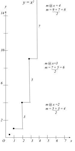
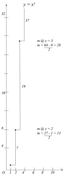
Here are more details. We can find a slope for x2 very simply and accurately by averaging forward and backward slopes, as you see from this graph. However, another similar graph tells us we cannot get the current value of the slope that way for x3. Why? It is because the curve x2 is changing 3, 5, 7, 9. You can get that either from the table or the graph. It is changing 2 each time. The curve x2 has a fundamental acceleration of 2. Therefore we can average in one step. The average of 5 and 7 is 6, which is the slope at x=3. But the curve x3 is changing 7, 19, 37. It appears we cannot average.
The modern calculus tells us this is why we have to go to zero. We cannot average forward and backward slopes with most functions, therefore we have to solve by going to zero. But that is false. With x3 we do not have to go to zero any more than we did with x2. We can find a derivative with a simple average. Like this.
Since x3 is changing 7, 19, 37, it has a fundamental acceleration of 6n (where n=1, 2, 3). You can see that in the last two lines in the table above. That being the case, our acceleration could be written as this series:
1, 1 + 6, 1 + 12, 1 + 18, 1 + 36...
That is where the numbers 1, 7, 19, 37 come from. So, if we want to find the slope at 3, say, that will be between the numbers 19 and 37. Just consult the graph. It has been shown that we cannot average 19 and 37 directly, because that would give us the number 28, which is not the current slope. But since the curve is is achieved by a 1+ series, we can subtract the one away from each term. If we do that, then our forward and backward slopes at x=3 will be 18 and 36, in which case we can find the current slope by averaging. (18 + 36)/2 = 27. That is the current slope at 3. So we could find a slope just by averaging, even with an acceleration of 6n.
You will say, “Wait, you just changed your curve by doing that. You just proved that changing the curve was forbidden, then you did it. You subtracted 1 away from your series, and you now have this series:
Δx3 = 6, 18, 36, 60, 90
Those are the rates of change for 0, 6, 24, 60, 120, 210, not x3 = 1, 8, 27, 64, 125, 216.”
True, but the curve 0, 6, 24, 60, 120, 210 is still an acceleration of 6n, therefore it is an acceleration above x2, therefore you CAN find an average acceleration for powers above 2. You cannot find it just by adding two numbers and dividing by 2, but you can find it. In this case, it is the forward slope minus 1 plus the backward slope minus 1, over 2. It is still an average, it is still very simple, and it doesn't require using a limit.
m@(x,y) = {[Δy@(x+1)]
– 1} + {[Δy@(x)] – 1}
2
The same analysis applies to x4:
m@(x,y) = {[Δy@(x+1)]
– 12} + {[Δy@(x)] – 12}
2
Because we can average forward and backward slopes like this with a general equation, it means the process is not an accident or push.
Δx5 = 1, 31, 211, 781, 2101, 4651, 9031
m@(x,y) = {[Δy@(x+1)]
– (10x2 + 1)} + {[Δy@(x)] – (10x2 +
1)}
2
We can average powers above 2 because they are constant. They are constant not as the power 2 is constant: the power 2 is constant at the first rate of change. But all simple powers are constant in that they increase in a consistent manner, by a process that can be broken down. We can see that right from the tables. If we take enough changes of any power, we see that it is constant at a fundamental level. That is what 6, 6, 6, 6 is telling us about x3. Two rates down, it is constant. Therefore it is constant. That was my point in a recent paper on “variable” acceleration. Cubed acceleration is not really variable. It is constant. It can be averaged, if you do it in the right way. It is a consistent increase, therefore it can be analyzed in a straightforward manner, as we are doing here. We do not need limits, we can just use simple number relations.
Although it has been shown we can average forward and backward slopes with all powers, the slope equations get very complicated as we advance into the higher powers. We also encounter a problem with finding slopes for values of x near 1, since we are subtracting large numbers from our Δy's. This means we need a better way to generalize our slope equation.
We will pull the general equation straight from the tables. We will start with the smaller powers. Since x3 is changing 7, 19, 37, it has a fundamental acceleration of 6n (where n=1, 2, 3). You can see that in the last two lines in the table above. Since x2 has a fundamental acceleration of 2, the fundamental acceleration of x3 is 3 times that of x2 over each interval. Six is three times two. We can write that as f x3 = 3x2, where f means fundamental acceleration.
If we are physicists, or logical people of any stripe, that proof of the derivative of x3 is much preferable to the current one. We do not go to zero, we do not talk of limits or functions or infinitesimals or any of that. We pull the general derivative equation straight from a table of differentials, and in doing so we see right where all the numbers are coming from. Now we just need to generalize that equation. We can do that by analyzing other powers. By studying The Algorithm, we find that all other powers obey the same relationship we just found between x2 and x3.
f xn = nxn-1
The
differentials themselves give us the derivative equation for
powers. This means we do not need any other proof of it. A table
of differentials is all the proof we need. It is a proof by “show
me.” You want me to prove that the derivative
equation for powers is:
f
xn
= nxn-1,
there are the numbers sitting right next to
each other. If you require a proof beyond that, we must call you
a confused and meddlesome person, and we recommend you go into
set theory, where you can write thousand-page books proving
tautologies (while ignoring much greater real problems sitting on
your desk).
A reader may ask, “We can write the series 0, 6, 24, 60, 120, 210... as x3 – x, and you have shown that both the curve x3 – x and the curve x3 can be written as accelerations of 6n. By your abbreviated and direct proof, both curves should have a derivative of 3x2. But they do not. The derivative of x3 – x is 3x2 – 1. How do you explain that?”
There is no need to show that the proofs are wrong. It is true that the derivatives are different for x3 – x and x3, but that difference can be shown and generalized without using limits. In this case, the difference is caused by the first term in the series. The first term in one series is 1 different from the other, and so is the derivative. So the difference in equations can be shown by simple demonstration, or by pointing to a table. It doesn't require limits or difficult proofs.
All calculus questions can be answered by studying the tables, since the tables supply the actual number relations that generate the calculus. Fundamentally, calculus is about these number relations, not about limits or approaches to zero.
Because the calculus is not about limits and can be proved without limits, it cannot find solutions at points or instants. MM's method differs from the modern calculus not only in its simplified proofs, but in its definitions. Because Δx is always 1 and cannot go below one, our derivatives and solutions are always found over a defined interval of 1.
Instantaneous velocities and accelerations are impossible, as are point particles and all other solutions at points. This solves many of the problems of QED and General Relativity. It solves renormalization directly, since the equations are never allowed to become abnormal to begin with. And it disallows "mass points" in the field equations. If you cannot have math at a point, you cannot have mass at a point.
Modern physicists have been fooled by the calculus into thinking they can or should be able to do things they simply cannot do. My correction to the calculus disabuses them of this mistaken notion. They have had problems with points in their math and their fields because points do not exist, in either math or fields. Only intervals exist. Only intervals can be studied mathematically. This is why they call it the differential calculus. It is a calculus of differentials, and differentials are always intervals. Just check the epsilon/delta proof. It is defined by differentials, not points. Mathematicians at all levels and in all centuries always seem to forget that whenever it is convenient.
Part Three - The Rest of the Groundwork
The next item of the new structure concerns "rate of change" and the way the concept of change applies to the cardinal number line. Rate of change is a concept that is very difficult to divorce from the physical world. This is because the concept of change is closely related to the concept of time. This is not the place to enter a discussion about time; suffice it to say that rate of change is at its most abstract and most mathematical when we apply it to the number line, rather than to a physical line or a physical space. But the concept of rate of change cannot be left undefined, nor can it be taken for granted. The concept is at the heart of the problem of the calculus, and therefore we must spend some time analyzing it.
MM has already shown that the variables in a curve equation are cardinal numbers, and as such they must be understood as delta variables. In mathematical terms, they are differentials; in physical terms, they are lengths or distances. This is because a curve is defined by a graph and a graph is defined by axes. The numbers on these axes signify distances from zero or differentials: (x – 0) or (y – 0). In the same way the cardinal number line is also a compendium of distances or differentials. In fact, each axis on a graph may be thought of as a separate cardinal number line. The Cartesian graph is then just two number lines set zero to zero at a 90o angle.
This being true, a
subtraction of one number from another—when these numbers
are taken from Cartesian graphs or from the cardinal number
line—is the subtraction of one distance from another
distance, or one differential from another. Written out in full,
it would look like this:
ΔΔx = Δxf
- Δxi
Where Δ xf is the
final cardinal number and Δxi is the initial
cardinal number. This is of course rigorous in the extreme, and
may seem pointless. But be patient, for we are rediscovering
things that were best not forgotten. This equation shows that a
cardinal number stands for a change from zero, and that the
difference of two cardinal numbers is the change of a change. All
we have done is subtract one number from another and we already
have a second-degree change.
Following this strict method, we find that any integer subtracted from the next is equal to 1, which must be written ΔΔx = 1. On a graph each little box is 1 box wide, which makes the differential from one box to the next 1. To go from one end of a box to the other, you have gone 1. This distance may be a physical distance or an abstract distance, but in either case it is the change of a change and must be understood as ΔΔx = 1.
Someone might interrupt at this point to say, "You just have one more delta at each point than common usage. Why not simplify and get back to common usage by canceling a delta in all places?” We cannot do that because then we would have no standard representation for a point. If we let a naked variable stand for a cardinal number, which MM has shown is not a point, then we have nothing to let stand for a point. It is necessary to clear up the problem as follows: we must let x and y and t stand for points or instants or ordinals, and only point or instants or ordinals. We must not conflate ordinals and cardinals, and we must not conflate points with distances. We must remain scrupulous in our assignments.
Next, it might be argued that we can put any numbers into curve equations and make them work, not just integers. True, but the lines of the graph are commonly integers. Each box is one box wide, not ½ a box or e box or π box. This is important because the lines define the graph and the graph defines the curve. It means that the x-axis itself has a rate of change of one, and the y or t-axis also. The number line itself has a rate of change of one, by definition. None of my number theory here would work if it did not.
For instance, the sequence 1, 1, 1, 1, 1, 1.... describes a point. If you remain at one you don’t move. A point has no RoC (rate of change). Its change is zero, therefore its RoC is zero. The sequence of cardinal integers 1, 2, 3, 4, 5…. describes motion, in the sense that you are at a different number as you go down the sequence. First you are at 1, then at 2. You have moved, in an abstract sense. Since you change 1 number each time, your RoC is steady. You have a constant RoC of 1. A length is a first-degree change of x. Every value of Δx we have on a graph or in an equation is a change of this sort. If x is a point in space or an ordinal number, and Δx is a cardinal number, then ΔΔx is a RoC.
MM also stresses that the cardinal number line has a RoC of 1 no matter what numbers you are looking at. Rationals, irrationals, whatever. Some may argue that the number line has a RoC of 1 only if you are talking about the integers. In that case it has a sort of “cadence,” as it has been suggested to me. Others have said that the number line must have a RoC of zero, even by my way of thinking, since it has an infinite number of points, or numbers. There are an infinite number of points from zero to 1, even. Therefore, if you “hop” from one to the other, in either a physical or an abstract way, then it will take you forever to get from zero to one. But that is simply not true. As it turns out, in this problem, operationally, the possible values for Δx have a RoC of 1, no matter which ones you choose. If you choose numbers from the number line to start with (and how could you not) then you cannot ever separate those numbers from the number line. They are always connected to it, by definition and operation. The number line always “moves” at a RoC of 1, so the gap between any numbers you get for x and y from any equation will also move with a RoC of 1.
If this is not clear, let us take the case where you choose values for x1 and x2 arbitrarily, say x1 = .0000000001 and x2 = .0000000002. If you disagree with my theory, you might say, "My gap is only .0000000001. Therefore my RoC must be much slower than one. A sequence of gaps of .0000000001 would be very very slow indeed." But it wouldn’t be slow. It would have a RoC of 1. You must assume that your .0000000001 and .0000000002 are on the number line. If so, then your gap is ten billion times smaller than the gap from zero to 1. Therefore, if you relate your gap to the number line—in order to measure it—then the number line, galloping by, would traverse your gap ten billion times faster than the gap from zero to one. The truth is that your tiny gap would have a tiny RoC only if it were its own yardstick. But in that case, the basic unit of the yardstick would no longer be 1. It would be .0000000001. A yardstick, or number line, whose basic unit is defined as 1, must have a RoC of 1, at all points, by definition.
From all this you can see that has been defined is the rate of change so that it is not strictly equivalent to velocity. A velocity is a ratio, but it is one that has already been established. A rate of change, by my usage here, is a ratio waiting to be calculated. It is a numerator waiting for a denominator. MM defines one delta a change and two deltas a rate of change. Three deltas would be a second-degree rate of change (or 2RoC), and so on.
(The Algorithm section from the long are paper used to be here but was moved to the beginning in the calcsimp preface.)
Part Five - The Derivation
Now, let us
examine what the current value for the derivative is telling us,
according to my chart. If we have a curve equation, say
Δt
= Δx3
Then the derivative (y’ = nxn-1) is
Δt' =
3Δx2
From the new chart
{ΔΔΔx2 = 2, 2, 2, 2, 2, 2, 2, 2, 2, 2
ΔΔΔΔx3 = 6, 6, 6, 6, 6, 6, 6, 6}
it can be seen that
3ΔΔΔx2
= ΔΔΔΔx3
So, 3Δx2 =
ΔΔx3
[Deltas may be cancelled across these particular
equalities]*
And, Δt' = 3Δx2 = ΔΔx3
Δt = Δx3
Therefore, Δt' =
ΔΔt
The derivative is just the rate of change of our dependent variable Δt, the rate of change of a length or period. It is not the rate of change of a point or instant. A point on the graph stands for a value for Δt, not a point in space. The derivative is a rate of change of a length (or a time period).
* Why can we cancel deltas here? That is a very important question. Is a delta a variable? Is every delta equal to every other delta? The answer is that a delta is not a variable; and that every delta does not equal every other delta. Therefore the rules of cancellation are a bit tricky. A delta is not a free-standing mathematical symbol. You will never see it by itself. It is connected to the variable it precedes. A variable and all its deltas must therefore be taken as one variable. This would seem to imply that canceling deltas is forbidden. However a closer analysis shows that in some cases it is allowed. A variable and all its deltas stand for an interval, or a differential. At a particular point on the graph, that would be a particular interval. But in a general equation, that stands for all possible intervals of the variable. As you can see from my table, some delta variables have the same interval value at all points. Most don’t. High exponent variables with few deltas have high rates of change. However, all the lines in the table are dependent on the first line. Notice that each line could be read as, " If Δx = 1,2,3,etc., then this line is true." You can see that you put those values for Δx into every other line, in order to get that line. Each line of the table is just reworking the first line. Line three is what happens when you square line one, for instance. So that the underlying variable Δx is the same for every line on the table. Therefore, if you set up equalities between one line and another, the rates of change are relatable to each other. They are all rates of change of Δx. That is why you can cancel deltas here.
This all goes to say that if x is on both sides of the equation, you can cancel deltas. Otherwise you cannot.
Now
let's do that again without using what we already know from the
calculus. Let's prove the derivative equation logically just from
the chart without making any assumptions that the historical
equation is correct. Again, we are given the curve equation and a
curve on a graph. Δt = Δx3
We then look
at my second little chart to find Δx3 . We see
that the differential is constant (6) when the variable is
changing at this rate: ΔΔΔΔx3.
{ΔΔΔx2 = 2, 2, 2, 2, 2, 2, 2, 2, 2, 2
ΔΔΔΔx3 = 6, 6, 6, 6, 6, 6, 6, 6}
You will say, "Wait, explain that. Why did you go there on
the chart? Why do we care where the differential is constant?"
We care because when the differential is constant, the curve
is no longer curving over that interval. If the curve is no
longer curving, then we have a straight line. That straight line
is our tangent. That is what we are seeking.
Now let's show what 2ΔΔx = ΔΔΔx2 means. The equation is telling us "two times the rate of change of x is equal to the 2RoC of x2." This is somewhat like saying "twice the velocity of x is equal to the acceleration of x2." These equalities are just number equalities. They do not imply spatial relationships. For instance, if one says, “My velocity is equal to your acceleration,” this is not saying anything about our speeds. This is not saying that we are moving in the same way or covering the same ground. It is simply noticing a number equality. The number calculated for MM's velocity just happens to be the number you are calculating for your acceleration. It is a number relation. This number relation is the basis for the calculus. The table above is just a list of some slightly more complex number relations. But they are not very complex, obviously, since all we had to do is subtract one number from the next.
Next let's look again at our given equation, Δt = Δx3
What exactly is that equation telling us? Since the graph gives us the curve—defines it, visualizes, everything—we should go there to find out. If we want to draw the curve, what is the first thing we do? We put numbers in for Δx and see what we get for Δt, right? What numbers do we put in for Δx? The integers, of course. You can see that if we put integers in, then Δx is changing at the rate of one. We put in 1 first, and then 2, and so on. So Δx is changing at a rate of one. As proved above, we don't have to put in integers. Even if we put in fractions or decimals, Δx will be changing at the rate of one. It just won't be so easy to plot the curve. If Δx is changing at the rate of one, then Δt will be changing at the rate of Δx3. That is all the equation is telling us.
Now that we are clear on what everything stands for, we are ready
to solve.
We are given Δt = Δx3
We
find from the table 3ΔΔΔx2 =
ΔΔΔΔx3
We simplify 3Δx2
= ΔΔx3
We seek ΔΔt
We
notice ΔΔt = ΔΔx3 since we can
always add a delta to both sides**
We substitute ΔΔt
= 3Δx2
ΔΔt = Δt'
So
Δt' = 3Δx2
Now to explain the steps thoroughly: The final equation reads, in full: "When the rate of change of the length Δx is one, the rate of change of the length (or period, in this case) Δt is 3Δx2." The first part of that sentence is implied from my previous explanations, but it is good for us to see it written out here, in its proper place. For it tells us that when we are finding the derivative, we are finding the rate of change of the first variable (the primed variable) when the other variable is changing at the rate of one. Therefore, we are not letting either variable approach a limit or go to zero. To repeat, ΔΔx is not going to zero. It is the number one.
That is why you can let it evaporate in the denominator of the current calculus proof. In the current proof the fraction Δy/Δx (this would be ΔΔy/ΔΔx by my notation) is taken to a limit, in which case Δx is taken to zero, we are told. But somehow the fraction does not go to infinity, it goes to Δy. The historical explanation has never been satisfactory. It has been shown that it is simply because the denominator is one. A denominator of one can always be ignored.
** We were allowed to add deltas to both sides of the equation in this case because we were adding the same deltas. Deltas aren’t always equivalent, but we can multiply both sides by deltas that are equivalent. What is happening is that we have an equality to start with. We then give the same rate of change to both sides: so the equality is maintained.
The question that arises, is how does one know to seek ΔΔt in the above proof? The objective is to solve the problem without taking any assumptions from the current proof or use of the calculus. Why did one seek it? What does it stand for in the interpretation? What is happening on the graph or in real life that explains ΔΔt?"
The answer will complete this proof. By the very way the equation and the graph are set up,
it can be shown that it must be true that ΔΔx = 1. Given
that, what are we seeking? It is the tangent to the curve on the graph.
The tangent to the curve on the graph is a straight line
intersecting the curve at (Δx, Δt). Each tangent will
hit the curve at only one (Δx, Δt), otherwise it
wouldn't be the tangent and the curve wouldn't be a
differentiable curve. Since the tangent is a straight line, its
slope will be ΔΔt/ΔΔx. So we need an
equation that gives us a ΔΔt/ΔΔx for
every value of Δt and Δx on our curve. Nothing could
be simpler. We know ΔΔx = 1, so we just seek
ΔΔt.
ΔΔt/ΔΔx = ΔΔt/1
= ΔΔt
ΔΔt is the slope of the tangent
at every point on the curve on the graph.
If Δt = Δx3
Then ΔΔt = 3Δx2
Part Six - Application to Physics
The first part of our problem is solved, having found the derivative without calculus and having assigned its value to the general equation for the slope of the tangent to the curve. The next question would be whether we can assign this equation to the velocity at all "points on the curve". This is no longer a math question. It is a physics question. The answer appears to be "yes." ΔΔt/ΔΔx = ΔΔt = (Δt)'
Although t was made the dependent variable initially, but this is an arbitrary choice. If x was the dependent variable, then we would have had (Δx)' = ΔΔx/ΔΔt
So the derivative looks like a velocity.
But the velocity at the point on the graph is not the velocity at a point in space, therefore the slope of the tangent does not apply to the instantaneous velocity. It is the velocity during a period of time of acceleration, not the velocity at an instant.
It might be believed that by the methods above that one could continue to cancel deltas, in which case we will get ΔΔt/ΔΔx = Δt/Δx = t/x. If the Δt's are equal then the t's are equal, and so on." This process would be incorrect.
Notice that the equation x/t doesn't even describe a velocity. It is a point over an instant. That is not a velocity. It is not even a meaningful fraction. It has been shown that t in that case is really an ordinal number. You cannot have an ordinal as a denominator in a fraction. It is absurd. In reducing that last fraction, you are saying that 5 meters/5 seconds would equal the fifth meter mark over the fifth second tick. But the fifth meter mark is equivalent to the first meter mark and the hundredth meter mark. And the fifth tick is the same as every other tick. Therefore, MM could say that 5 meters/5 seconds = 5th mark/5th tick = 100th mark/ 7th tick. Gobbledygook.
Furthermore, such a method of cancellation is not allowed. Certain deltas across equalities were canceled previously under strictly analyzed circumstances (x was on both sides of the equation), but the cancelation being proposed is across a fraction. Simplifying a fraction by canceling a delta in the numerator and denominator is not the same as canceling a term on both sides of an equation. Obviously, ΔΔt/ΔΔx cannot equal Δt/Δx, since the derivative is not the same as the values at the point on the graph. The slope of a curve is not just Δy/Δx. A delta does not stand for a number or a variable, therefore it does not cancel in the same ways. It sometimes cancels across an equality, as has been shown. But the delta does not cancel in the fraction ΔΔt/ΔΔx, because Δt and Δx are not changing at the same rate. If they changed at the same rate, then we would have no acceleration. The deltas are therefore not equivalent in value and cannot be cancelled.
Given that velocity is not an
instantaneous velocity, it must be the velocity over some
interval. It has just been shown that it is not the velocity of the
interval Δxfinal - Δxinitial because that only applies if
the curve is a straight line. It is the interval of velocity
over the nth interval of ΔΔx, where ΔΔx =
1. [If t were the independent variable, then the interval would
be ΔΔt.] Again, ΔΔt/ΔΔx is
the velocity equation, according to our given equation. Therefore
the velocity at a given point on the graph (Δxn,
Δtn) is the velocity over the nth interval ΔΔx.
This is straightforward since the velocity equation tells us that itself:
the denominator is the interval. Each interval ΔΔx is
one, but the velocity over those intervals is not constant, since
we have an acceleration. The velocity we find is the velocity
over a particular subinterval of Δx. The subinterval of Δx
is ΔΔx. The velocity may be written this way:
Δt'
/ ΔΔx
We have not gone to a limit or to zero; we have gone to a subinterval—the interval directly below the length and the period. What this means is that our basic intervals or differentials are Δx and Δt. But if we have a curve equation, we have an acceleration or its mathematical equivalent. If we have an acceleration, then while we are measuring distance and period, something is moving underneath us. We have a change of a change. A rate of change. Our basic intervals are undergoing intervals of change. Not that hard to imagine. It happens all the time. While I am walking in the airport (measuring off the ground with my feet and my watch) I step onto a moving sidewalk. The ground has changed over a subinterval. It changes over only one subinterval, so I feel acceleration only over this subinterval. Once I achieve the speed of the sidewalk, my change stops, the subinterval ends, and I am at a new constant velocity. The subinterval is not an instant, it is the time(beginning of change) to the time(end of change). But in constant acceleration, I would be stepping onto faster sidewalks during each subsequent subinterval, and I would continue to accelerate.
Thus the subinterval is not an instant. It is a definite period of time or distance, and this time or distance is given by the equation and the graph. As has been exhaustively shown, the subinterval in any graph where the box length is one and the independent variable is Δx is simply ΔΔx = 1. If we assign the box length to the meter, then ΔΔx = 1m. If we find the velocity "at a point," then we must assign that velocity to the interval preceding that point. Not an infinitesimal interval, but the interval 1 meter. If we then assign that velocity to a real object at a point in space, an object we have been plotting with our graph and our curve, then the velocity of the object must also be assigned to the preceding one-meter interval.
Since a real object does not accelerate by fits and starts and nor does the curve on the graph, it should be able to find the velocity at any fractional point, in space or on the graph. This is possible, but the value achieved will apply to the interval, not the instant. You can find the velocity at the value Δx = 5m or Δx = 9.000512m or at any other value, but any velocity will apply to the metric interval preceding the value.
In the example, a meter is not very precise, but that does not mean that the interval cannot be smaller. Just assign your box length to a smaller magnitude. If you let each box equal an angstrom, then the interval preceding your velocity is also an angstrom. However, notice that you cannot arbitrarily assign magnitude. That is, if you are actually measuring your object to the precision of angstroms, fine. You can mirror that precision on your graph. But if you are not being that precise in your operation of measurement, then you can’t assign a very small magnitude to your box length just because you want to be closer to an instant or a point. Your graph is a representation of your operation of measurement. You cannot misrepresent that operation without cheating. It would be like using more significant digits than you have a right to.
This means that in physics, the precision of your measurement of your given variables completely determines the precision of your velocity. This is logically just how it should be. We should not be able to find the velocity at an instant or a point, when we cannot measure an instant or a point. An instantaneous velocity would have an infinite precision. We have a margin of error in all measurement of length and time, since we cannot achieve absolute accuracy. But heretofore we expected to find instantaneous velocities and accelerations, which would imply absolute accuracy.
Part Seven - The Second Derivative—Acceleration
As a final step, it can be shown that the second derivative is also not found at an instant. There is no such thing as an instantaneous acceleration, any more than there is an instantaneous velocity. What we seek for the acceleration at the point on the graph is this equation: Δt'' = ΔΔΔt/ΔΔx
Acceleration is
traditionally Δv/Δt. By current notation, that is
(ΔΔx /Δt)/ Δt. By my notation of extra
deltas, that would be [Δ(ΔΔx)/ΔΔt]
/ ΔΔt . My variables have been upside down this whole
paper, thus finding slope and velocity as t/x
instead of x/t. So flipping that last equation
[Δ(ΔΔt)/ΔΔx]
/ ΔΔx
As we have found over and over, ΔΔx
= 1, that equation reduces to ΔΔΔt.
For the acceleration we seek ΔΔΔt. The
denominator is one, as you can plainly see, which means we are
still seeking ΔΔΔt over a subinterval of one,
not an interval diminishing to zero or to a limit.
We are
given Δt = Δx3
We find from the table
3ΔΔΔx2 = ΔΔΔΔx3
We simplify 3ΔΔx2 = ΔΔΔx3
We
seek Δt'' or ΔΔΔt
We notice ΔΔΔt
= ΔΔΔx3 since we can add the same
deltas to both sides
We substitute 3ΔΔx2
= ΔΔΔt
Back to the table 2ΔΔx =
ΔΔΔx2
Simplify 2Δx = ΔΔx2
Substitute once more 6Δx = ΔΔΔt
At
Δx = 5, ΔΔΔt = 30
The subinterval for the acceleration is the same as the
subinterval for velocity. This subinterval is 1.
Summation
The proof is complete. Newton’s analysis was wrong, and so was Leibniz’s. No fluxions are involved, no vanishing values, no infinitesimals, no indivisibles (other than zero itself). Nothing is taken to zero. No denominator goes to zero, no ratio goes to zero. Infinite progressions are not involved. Even Archimedes was wrong. Archimedes invented the problem with his analysis, which looked toward zero 2200 years ago. All were guilty of a misapprehension of the problem, and a misunderstanding of rate of change. Euler and Cauchy were also wrong, since there is no sense in giving a foundation to a falsehood. The concept of the limit is historically an ad hoc invention regarding the calculus: one which may now be jettisoned. My redefinition of the derivative as simply the rate of change of the dependent variable demands a re-analysis of almost all higher math.***
The entire mess was built on one great error: all these mathematicians thought that the point on the graph or on the mathematical curve represented a point in space or a physical point. There was therefore no way, they thought, to find a subinterval or a differential without going to zero. But the subinterval is just the number one, as was shown. That was the first given of the graph, and of the number line. The differential ΔΔx = 1 defines the entire graph, and every curve on it. That constant differential is the denominator of every possible derivative—first, second or last. The derivative is not the limit as Δx approaches zero of Δf(x)/Δx. It is the value Δf(x)/1.
And this is precisely why the Umbral Calculus works. The current interpretation and formalism of the Calculus of Finite Differences is so complex and over-signed that it is difficult to tell what is going on. But my simple explanation of it above shows the groundwork clearly, even to those who are not experts in this subfield. Once you limit the Calculus of Finite Differences to the integers, build a simple table, and refuse to countenance things like forward differences and backward differences (which are just baggage), the clouds begin to dissipate. You give the constant differential 1 to the table, not arbitrarily, but because the number line itself has a constant differential of 1. We have defined the number 1 as the constant differential of the world and of every possible space. Mathematicians seem apt to forget it, but it is so. Every time we apply numbers to a problem, we have automatically defined our basic differential as 1. What this means, operationally, is that in many problems, exponents begin to act like subscripts, or the reverse. To see this, go back to the table above. Because the integer 1 defines the table and the constant differentials on it, the exponents could be written as subscripts without any change to the math.
Once we have defined our basic differential as 1, we cannot help but mirror much of the math of subscripts, since subscripts are of course based on the differential 1. Unless you are very iconoclastic, your subscript changes 1 each time, which means your subscript has a constant differential of 1. So does the Calculus of Finite Differences, when it is used to replace the Infinite Calculus and derive the derivative equation as was done here. Therefore it can be no mystery when other subscripted equations—if they are explicitly or implicitly based on a differential of 1—are differentiable.
Beyond this, by redefining the problem completely, it proves that instantaneous values are a myth. They do not exist on the curve or on the graph. Furthermore, they imply absolute accuracy in finding velocities and accelerations, when the variables these motions are made of—distance and time—are not, and cannot be, absolutely accurate. Instantaneous values do not exist even as undefined mathematical concepts in the calculus, since they were arrived at by assigning diminishing differentials to points that were not points. You cannot postulate the existence of a limit at a “point” that is already defined by two differentials, (x - 0) and (y - 0).
This was achieved with an algorithm that is simple and easy to understand. Calculus may now be taught without any mystification. No difficult proofs are required; nothing must be taken on faith. Every step of my derivation is capable of being explained in terms of basic number theory, and any high school student will see the logic in substituting values from the chart into curve equations.
[As proof that the calculus does not go to a limit, an infinitesimal, or approach zero, see "A Correction to Newton's Equation a=v2/r". There, the equation on the Moon is used to show that the acceleration of the Moon due to the Earth is not an instantaneous acceleration. In other words, it does not take place at an instant or over an infinitesimal time. MM actually calculates the real time that passes during the given acceleration, showing in a specific problem that the calculus goes to a subinterval, not a limit or infinitesimal. That subinterval is both finite and calculable in any physical problem. In other words, MM finds the subinterval that acts as 1 in a real problem. MM finds the value of the baseline differential.]
[In the section at the end of the paper A Study of Variable Acceleration, MM proves that calculus is fundamentally misunderstood to this day by analyzing a textbook solution of variable acceleration. He shows that the first integral is used where the second derivative should be used, proving that scientists don't comprehend the basic manipulations of the calculus. Furthermore, he shows that calculus is taught upside-down, by defining the derivative in reverse.]
*** For example, my correction to the calculus changes the definition of the gradient, which changes the definition of the Lagrangian, which changes the definition of the Hamiltonian. Indeed, every mathematical field is affected by my redefinition of the derivative. MM has shown that all mathematical fields are representations of intervals, not physical points. It is impossible to graph or represent a physical point on any mathematical field, Cartesian or otherwise. The gradient is therefore the rate of change over a definite interval, not the rate of change at a point.
Symplectic topology also relies upon the assumptions overturned in this paper. If points on a Cartesian graph are not points in real space, then quantum mechanical states are not points in a symplectic phase space. Hilbert space also crumbles, since the mathematical formalism cannot apply to the fields in question. Specifically, the sequence of elements, whatever they are, does not converge into the vector space. Therefore the mathematical space is not equivalent to the real space, and the one cannot fully predict the other. This means that the “uncertainty” of quantum mechanics is due (at least in part) to the math and not to the conceptual framework. That is to say, the various difficulties of quantum physics are primarily problems of a misdefined Hilbert space and a misused mathematics (vector algebra), and not problems of probabilities or philosophy.
In fact, all topologies are affected by this paper. Elementary topology makes the same mistake as the calculus in assuming that a line in R2 represents a one-dimensional subspace. But it was just shown that a line in R2 represents a velocity, which is not a one-dimensional subspace. I proved in section 1 above that a point in R2 was already a two-dimensional entity, so a line must be a three-dimensional subspace. In R3 a line represents an acceleration. In R4 a line represents a cition (Δa). Since velocity is a three-dimensional quantity—requiring the dimensions y and t, for instance, plus a change (a change always implies an extra dimension)—it follows that a line in Rn represents an (n+1) dimensional subspace.
This means that all linear and vector algebras must be reassessed. Tensors are put on a different footing as well, and that is a generous assessment. Not one mathematical assumption that relies on the traditional assumptions of differential calculus, topology, linear algebra, or measure theory is untouched by this paper.
Another Fatal Flaw in the Historical Derivation of Calculus
The historical proof of the calculus bids us imagine some infinite series of shrinking numbers. It lets this series approach a limit. This limit is usually conceived of as a point. As an example let us imagine a sphere. Let the radius of the sphere be our given number. Now, let our sphere begin shrinking. The given number will get smaller, of course. The calculus supposes that as the given number gets smaller it gets closer to zero. It approaches zero. This implies that our shrinking sphere will physically approach a limit or a zero—that it will approach being a point. But it won’t. A shrinking sphere will not approach a point, not physically, metaphysically, mathematically, conceptually, really, or abstractly. This is why:
Size is a relative term. It is relative to other things and other times. You may be smaller than another thing, or smaller than you were yesterday, but other than that “small” has no meaning. A shrinking balloon has a limit. You can only let so much air out. It can’t get smaller than a deflated balloon. But if you take a sphere in physical or mathematical space and treat it only as structure, then there is no upper or lower limit on size. You can make it infinitely large or infinitely small. Large and small are opposite directions in extension, but they are the same conceptually. Just as a thing can go on expanding forever it can go on shrinking forever. Zero is precisely as far away as infinity. An infinite regression “toward” zero is exactly the same mathematically as an infinite progression toward infinity.
Most people have a somewhat easier time imagining a large infinity than a small infinity. Especially since we are not talking about a negative infinity or negative numbers here at all. We are talking about a regress toward zero. Smaller and smaller fractions, or the like. Just as a large number does not really ever approach infinity, a small positive number does not really approach zero. Any infinite progression or regression does not approach ending. It does not end, therefore it cannot logically approach ending.
Everything we have said here applies to “size” in general, not just to material or physical size. Let us subtract out all the physical content from the discussion above. Let the numbers be numbers alone, and not refer to any physical parameter like length. We still have an inherent concept of size that we cannot subtract out. Numbers have size no matter how abstract we make them. Two is bigger than one in pure math as well as in applied math. If so, then let us ask, “If we move from 2 to 1, have we approached zero?” An exact analogy is the question, “If we move from 2 to 3, have we approached infinity?”
Of course, if we are talking about integers then we have no exact analogy: the answer to the first question is yes and the second no, since obviously the next smallest integer after 1 is 0. But in the second question, we are infinitely far away from infinity at 2, and we are infinitely far away from infinity at 3. We have not approached infinity. At the highest number we can imagine, we are still infinitely far away from the end of the series of integers, by definition. In fact, if we have approached the end of the series, then the series is not infinite.
Next, let us leave integers, since some will invoke Cantor to start inserting doubts into my reasoning so far. Let us move to real numbers, which have a higher order of infinity, for those who believe in such things. Let us ask the two questions again. “If we start at 1 and move down, have we approached zero?” And, “If we start at 1 and move up, have we approached infinity?” It is clear that both questions are basically equivalent. We are dealing with an infinite series in either case. Neither series can possibly end, by definition. In fact, the proof of the calculus depends on using an infinite series. If a Cantorian or anyone else proved that a series actually had an end, then it would not be an infinite series, and it would not be the series the calculus is talking about. The calculus applies, axiomatically, to infinite series.
If this is so, then an infinite series of progressively smaller numbers does not in fact approach zero. The smallest number you can think of is still infinitely far away from zero. Therefore it is no closer to zero than 1 is, or a million billion.
All this is hard to imagine for some, since zero is not just like infinity in other ways. Zero has a slot on the number line. We reach it all the time in normal calculations. But we never reach infinity in normal calculations, and it has no slot on the number line. Zero is a limit we can point to on a ruler; infinity is not a limit we can point to on a ruler. For this reason, most people, or perhaps all people, have not yet seen that an infinite regression does not approach zero. Zero is not logically approachable by an infinite series of diminishing numbers. A diminishing series either approaches zero, or it is infinite. It cannot be both.
Therefore, the first postulate of the calculus is a contradiction. Not a paradox, a contradiction. Meaning that it is false. The calculus begins, “Given an infinite series that approaches zero….” But you cannot be given an infinite series that approaches zero.
Some pre-calculus problems get around this problem by summing the series. The ancient Greeks solved problems with infinite series, such as the paradoxes of Zeno (e.g. Achilles and the Tortoise), by summing the series. This has been seen as a sort of pre-calculus, and rightly so, since it deals with both infinite series and limits. But when a series is summed, it no longer matters whether or not the series “approaches” the limit or not. It is beside the point. It simply does not matter whether the series actually reaches or approaches the limit, not in a physical sense nor a mathematical sense. All that is necessary is to show that the sum cannot exceed the limit. Since this is so, it may logically be assumed that the sum does indeed approach the limit; and what is more, that the sum reaches it. However, the terms in the series do not. The terms in the series do not approach or reach the limit.
In post-Newtonian math, it has been the custom to give a foundation to the derivative, and thereby to the differential calculus, by first assuming an infinite series and then letting it approach a limit. The wording is normally something like that was started off this section, but this proof is not a proof of any integral or of the integral calculus. That is to say, we are not dealing with any summations at this point in the historical proof. Rather, the proof is a proof that determines the derivative. Only later do we use the derivative to define the integral and give a foundation to the integral calculus.
Therefore, when the proof of the derivative lets the series approach a limit, it is quite simply wrong to do so. The terms in the series do not approach the limit; only the sum of the series approaches the limit. In differential calculus, we are not dealing with sums. We are dealing with differentials, which are simply numbers gotten from differences (gotten by subtraction).
To be even more specific, the proof of the derivative, and of the differential calculus—as taught in contemporary courses—starts with a given differential. We are usually given a curve. We take a differential from the curve, x2 – x1 for instance. We then let that differential diminish by choosing further x’s that are closer and closer to x2. We then mathematically monitor what is happening to y differentials as the x differentials diminish. We want to know what happens when the x differential hits the limit at the point x2. So it is clear that summations or sums have absolutely nothing to do with differential calculus. We are not summing any series of x’s. We are following diminishing x’s, which are individual terms in the series. MM has shown above that these terms do not in fact approach the limit. Therefore the proof fails.
A member of the status quo will argue that this is just caviling—inventing problems. He will say, “It is clear that a diminishing series, and the terms in that series, do approach the limit, or zero in the case you have given. To show this, all one has to do is point at the curve. If we are taking smaller and smaller differentials, then of course those differentials are getting closer to x2. Look at the line itself. The distance is getting shorter, so x1 must be getting closer to x2. That is all the proof is claiming.”
But notice that my antagonist is now using a physical definition of distance. When one attacks it on physical grounds, the status quo claims that calculus is pure math, unsullied by physics. If one attacks it on logical grounds, the status quo hides behind physical statements. It points to the line, showing me that the line is shorter. But it is showing a length, and a length is a parameter. A length is not pure math.
To answer is this: Yes, the segment of the curve gets shorter as the differential diminishes. But what is this segment of the curve? Over any interval, the drawn curve or mathematical curve is a summation. The complete curve is an overlay of all possible variables in the problem. A segment of this curve is an overlay of all possible variables over the given interval. The curve, and its length, has nothing to do with the individual terms in the series of differentials. What we are concerned with in the differential calculus, and in the proof in question, are the individual terms in the infinite series, not the summation of these terms. So that showing that the length of the curve gets shorter is not to the point. It is a misdirection in argument.
The important point—the one that really matters—is the one that is set forth above. The terms in the infinite series do not approach zero or the limit or the point. The terms in the series in the question at hand are differentials, and they do not approach the limit. They are always infinitely far away from it, as long as “far” is understood in mathematical terms. Therefore it is meaningless to let a differential approach a limit. Differentials do not approach limits, by definition and all the rules of logic.
A Study of Variable Acceleration
Abstract:
Analyzed here is a textbook solution of variable acceleration, showing that it is incorrect in both method and answer. It is incorrect because it is solved improperly with integration when it would be easier and more transparent to solve with the second and third derivatives.This will show how calculus is taught upside down.
[Apparently many readers have been mystified by this section. They do not comprehend my method, and assume MM wrote it standing on his head. But MM sticks to it for in his opinion, it is far easier and far more transparent to solve for distance using the third derivative here than by integrating. If you penetrate this paper, some important scales will fall from your eyes.]
Previously in this paper MM has shown many problems with the modern calculus. In this paper MM will show problems in applying the calculus to variable acceleration. To do this, MM will follow a physics textbook solution line for line.
To start, we must ask what we mean by a variable acceleration. It could mean two things. One, it could mean that we were speeding up and slowing down, so that our change in velocity was not constant. That is not what is meant here, rather this is an acceleration represented by a power of 3 or more, as in the curve equation x = t3. That means that you take a constant acceleration and then accelerate it. For example, you take your car out on the highway and press down on the gas at a constant rate. If your foot and engine work like they should, you will have created a constant acceleration. Now, take that whole stretch of highway, suck it up into a huge alien spacecraft, and accelerate the spacecraft out of orbit, in the same direction the car is going. The motion of the car relative to the earth or to space is now the compound of two separate accelerations, both of which are represented by t2. So the total acceleration would be constant, not variable, but it would be represented by t4. This is what MM is calling a “variable acceleration” here. It is not really variable, it is just a higher order of change.
The acceleration would be represented by t3 if the alien spacecraft had a constant velocity instead of a constant acceleration. An acceleration is two velocities over one interval, so t3 is three velocities over one interval. Or, it is three changes in x over one defined interval, say one second. We can write that as either three x's or three t's, but it is common usage to use three t's in the denominator instead of three x's in the numerator.
The cubed acceleration can also be created in a car, by increasing your pressure on the gas pedal at a constant rate of increase. This will cause a cubed acceleration in the first few seconds.
In engineering, a higher order acceleration like this is called a “jerk” (though it is usually applied to a negative acceleration, as in a jerk to a stop). MM calls the positive acceleration a cition in my first paper on the derivative, from the Latin “citius”. As in the Olympics motto “citius, altius, fortius”: faster, higher, stronger.
Because this sort of acceleration is often called a variable acceleration in physics textbooks, most people seem to think it isn't constant, and therefore can't be averaged like the squared variable. But higher powers can be constant, if they are created by a constant process like the one MM proposed above with the car and the spacecraft. If the car and spacecraft are both accelerating at a constant rate, the higher power total acceleration will also be constant. Just because an acceleration has a power greater than two does not mean it isn't constant. We will see how important this is below.
Saying that acceleration is constant does not mean that we can average the velocity because the velocity is accelerating itself, so we cannot find the velocity at a given time by averaging. Constant acceleration means that it increases at a consistent rate and is not fluctuating, thus we have to take the second derivative, not the first..
Now let us look at all the problems encountered by modern mathematicians in trying to analyze this situation. In physics textbooks, the chapter on velocity and acceleration normally comes very early. In my textbook1, it comes in chapter 2. You don't need calculus for constant velocity, but for “instantaneous velocity” you do, so we get an entire subsection for that. To begin, we get a graph plotting x against t and are given a curve (but no curve equation).

In the next section, constant acceleration is covered, and we are given a graph that plots v against t, with a similar curve. And in the section after that, we find “variable” acceleration. We are given a graph that again plots v against t, with a curve.

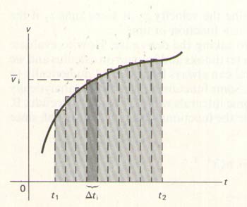
We should already have several questions. Since we are measuring the curvature of these curves with the graph, and finding tangents and areas beneath them, shouldn't our methods be analogous as we go from velocity to acceleration to variable acceleration? In other words, if we plot x against t in the first graph, shouldn't we plot x against t in all the graphs? Or, by another method, we would plot x against t in the first graph, v against t in the second, and a against t in the third. That would keep our method even and unchanged as we moved from one rate of change to the next.
Instead, we find the textbook plotting v against t when solving for a variable acceleration. This is not a quibble: it must be important, because the curve determines the tangent and the area under the curve. If you have a different curve, the tangent and the area are different, too. Well, plotting x against t will not give you the same curvature as plotting v against t or “instantaneous a” against t, will it? If we are going to differentiate or integrate, shouldn't we be careful to get the right curve?
Another problem. All textbooks apparently solve problems of variable acceleration with integration. But that is upside down. When solving with respect to t, you should differentiate down and integrate up. In other words, if you are given an acceleration and you want to find a velocity, you differentiate. The derivative of t2 is 2t, where t2 is the acceleration and 2t is the velocity. Conversely, to go from a velocity to an acceleration, you integrate. The integral of 2t is t2. But in textbooks, they integrate from a velocity graph, and find a velocity from a variable acceleration by integrating only once. Since a velocity is two steps from a variable acceleration, they should be seeking the second derivative, not the first integral.
To be even more specific, let me quote from the textbook:
If x is
given by x = At3
+ Bt, then v = dx/dt = 3At2
+ B. . .Then, since a = dv/dt, a = 6At.
What the authors are doing here is preparing you to integrate. They are showing you how differentiating works, and then preparing you to reverse it in the upcoming problem. You probably don't see anything wrong there, but, as MM pointed out about the exponential derivative, modern calculus is a jumble. What the textbook has done is take the first derivative and then the second, as you see, but they have called the first derivative of a variable acceleration a velocity and the second derivative a constant acceleration. That is backward. Just look at the equations: v = 3At2 + B? Since when can you write a velocity as a squared variable? Or, a = 6At? Isn't 6t a straight line on a graph? That isn't an acceleration.
My initial reaction was that this textbook author is just a nut, but by looking around me I have found that all of calculus now “works” this way. According to current wisdom, velocity is always supposed to be the derivative of distance, and acceleration the derivative of velocity, and that is what causes this horrible confusion. As I showed in previous papers, Wikipedia and most modern sources define the derivative like this, which is enough to raise Newton from the grave. He would tell you that when you are looking at the time variable, velocity is the derivative of acceleration, not the reverse. When manipulating t, you differentiate down and integrate up. When applying the calculus with respect to t, you differentiate down and integrate up.
Some will not see MM's point and will say, “What in the devil are you talking about? The first equation x = At3 + Bt is the distance. That is what the book means by 'x is given by'. That is what 'x equals' means!” But you need to pay attention. This is where it all comes out in the wash. The standard model and standard reply is wrong again, since the equation x = At3 + Bt is the curve equation on the graph, and it represents a variable acceleration. That equation is not x, that equation is the variable acceleration. You have been fooled by the “x=”.
Bear with me, please. Look closely at the equation x = At3 + Bt. The physical displacement x is not given by that equation. That equation applies to the graph only. It is telling you an x-distance from the y-axis at time t. The x in that equation tells you what x you are at, at the given value of t, but it does not tell you the distance traveled on the curve, since the curve is curving. To say it another way, x in a curve equation does not equal x in a physics equation. So x = At3 + Bt will not tell you a value for total distance traveled after t. If it did, we wouldn't need calculus at all, we could just read the value for x right off the graph, for any and all curves. But no, to find x you have to use physics equations, not curve equations. The equation x = At3 + Bt is a curve equation, and because it has a t3 in it, it must stand for a variable acceleration.
[Clarification, June 2015. By claiming that distance is the derivative of velocity MM realizes that he has shut most readers down when trying to understand this paper. We are all taught that velocity is the rate of change of distance, and in other papers MM even admits that is true. So they don't understand that here MM seems to be turning this upside down. They think it is crazy to say that when you are doing your calculus operations on the variable t, you actually differentiate down from velocity to distance. You take the derivative of t in the velocity equation to find the distance—which means that in this case, the distance is derivative of the velocity. If you follow MM's actual equations, you will see exactly what he means, and why he is right.
The difficult question is why this is so. It turns out it is because t is normally in the denominator. Being in the denominator in all equations of motion, t naturally acts upside-down to x as a matter of differentiation or integration. Not realizing this, the mainstream has butchered many of these manipulations when they are monitoring t. Any time they are finding anything “with respect to t” they are failing to take this into consideration.]
The entire modern interpretation of the calculus is upside down in this regard! To show this, let us look at the textbook solution of a specific problem:
Given a = 7m/s3 and 2s, find v final from rest.
v = ∫(7m/s3)tdt = (7m/s3)t2/2 = (3.5m/s3)t2 = 14m/s.
That solution looks like a fudge to me, from the start. If the moderns don't understand the foundations of the calculus, or how it works, it is unlikely they will be able to apply it in a logical and correct manner. In fact, the solution can't be right, because in the math they have taken one integral of time, to convert a variable acceleration to a velocity. Since the velocity is two steps of differentiation or integration away from the variable acceleration, in the differential table above or in real life, that solution can work only by some sort of accident or push or other miracle, but it does not work. That solution is not correct.
But first let us see why the textbook is integrating. We only have to look at its own explanation [this follows the quote above, explaining differentiation]:
The reverse process is also possible. If we are given the acceleration as a function of time, we can determine v as a function of time; and given v as a function of time, we can obtain the displacement, x.
The textbook integrates because it believes it is reversing the above process. But because as was just shown, their first process was upside down, this can't work. They thought they were going x→v→a with differentiation, so now they think they are going a→v→x with integration. But regarding the variable t, differentiation is the process a→v→x. Differentiation goes down, and integration goes up. They are trying to differentiate up and integrate down, when with t you have to do the reverse.
One more time, for good measure. We are given a curve equation, say y = x3. That is a curve equation, so it must stand for a curve. It does not stand for the point y or the distance y, since a point or distance y cannot curve. The only “y” it gives us is some vertical distance from the horizontal axis at some value of x. But that is not the solution for the distance traveled along the curve. Therefore it is not the solution to any physics problem. The equation y = x3 is not telling us a displacement, given an acceleration. It is telling us the acceleration.
Now let us solve the problem, without using integrals. We will start with the velocity. Then, we need to find the second derivative, since velocity is the second derivative of a variable acceleration. The second derivative of t3 is 6t, so while the time is changing by the cube, the velocity will be changing by 6's. You can see this clearly by taking the lines out of my differential tables:
Δx3
= 1, 8, 27, 64, 125, 216, 343
ΔΔx3
= 1, 7, 19, 37, 61, 91, 127
ΔΔΔx3
= 6, 12, 18, 24, 30, 36, 42
ΔΔΔΔx3
= 6, 6, 6, 6, 6, 6
The first line is the cubed acceleration, the second is the first rate of change of that acceleration, and the third is the second rate. The second line is (a sort of) first derivative of the first line, and the third line is (a sort of) second derivative. We are straightening out the curve. So the third line gives us a velocity. You can see that it is changing the same amount in between numbers. The differential is constant. That is the definition of a velocity. You can see that the velocity is changing by 6's. Its rate of change is 6. In our current problem, its rate of change is 6t, and t is 2, so at t=2, its rate is 12. Again, you can see that right from the table. The second entry is 12. But we have an acceleration of 7, not 1, so we multiply by 7 and divide by 2 (to take into account the first halved interval). This gives us v = 42m/s.
v = ad2(t3)/2 = 3at
That is the new equation for velocity, given a cubed acceleration. This is logical since we can derive the current equation for normal (squared) acceleration in the same way. The current equation is v = at. Current textbooks don't derive that equation with calculus, they just take it as given or derive it from the classical equation a = v/t. But we can now expand it showing the derivative:
v = ad(t2)/2 = at
Since the derivative of t2 is 2t, we get the current equation. This means we can intuit the velocity equation for an acceleration of t4 as
v = ad3(t4)/2 = 24at/2 = 12at
And v = ad4(t5)/2 = 120at/2 = 60at
MM has shown a simple method for taking higher order acceleration equations straight from my table of differentials. No one has ever done this before, that he knows of. It is certainly not done presently, because, as shown, current textbooks solve with integration.
Let us look at the textbook's solution. They found v=14m/s, remember? MM found 42m/s. You may think they are right and MM is wrong, but MM can prove they are wrong very easily. An acceleration of 7m/s3 must be greater than an acceleration of 7m/s2, right? A cubed acceleration is the motion of an acceleration, so the distance traveled has to be greater. So let us solve the same problem for a = 7m/s2 instead of 7m/s3. Using current equations for constant acceleration, we find
v = at = 14m/s.
They found the same final velocity for 7m/s3 and 7m/s2. That is impossible. An object accelerated to a cube must be going faster at all t's than an object accelerated to a square. That much is clear to anyone, hopefully. So the textbook solution is a blatant fudge, one that doesn't even get the right answer.
We can also use the differential table to find the distance here. But first let use my velocity 42m/s to find a solution. Because our acceleration is constant (or consistent), we can tweek the old equations.
x = vft/2 = (3at)t/2 = 3at2/2 = 42m.
Going to the table, we see that the object is moving 6 during each interval of 1. That is what 6, 6, 6, 6 means. Since our acceleration is 7, we just multiply. In doing this, we are using the third derivative, like so:
x = a(d3t3)t2/4 = 42m
To find a distance from a cubed acceleration, we take the third derivative. We differentiate down three times.
Let me clarify that. Some have not understood what MM is doing here. They have complained that MM is treating the acceleration as a motion constant and thereby trying to average the velocity or distance over the elapsed time. That is not what is happening. When MM says that the object is moving 6 during each interval, MM should say subinterval. MM does not mean that the object is traveling 6 during each 1/7 of a second or something, the same distance over each equal time. No, my third derivative is telling us that the object is moving 6 for each constituent velocity, and a cubed acceleration is made up of three of those. You really have to study the tables to see what MM is doing, and no one has done that in centuries. The calculus hasn't been taught like that, so my simple manipulations seem mysterious.
Let us see what the textbook got:
To get the displacement, we use x2 = ∫ v(t)dt with v1 = 0, v2 = 14m/s, and t2 = 2s.
x2 = ∫(3.5m/s3)t2dt = (3.5m/s3)t3/3 = 9.33m
Again, let us check that by comparing it to the solution for the distance traveled after 2 seconds at 7m/s2. Everyone agrees that the equation x = at2/2 works for constant acceleration, so we find 14m. The textbook found a number less than that, therefore the textbook cannot possibly be correct. A cubed acceleration must give us more displacement after any amount of time than a squared acceleration.
MM has just proven that the textbook solution is a fudge, in both method and answer.
Conclusion: MM has shown in a direct manner that modern physicists and mathematicians do not know how to use the calculus. Anytime you see a scientist integrating down from accelerations to distances in this way, you know that madness is afoot. In the previous sections of this paper, MM has shown that the calculus is misdefined, and now it has been shown to be misused, even in simple problems. Nor is this an isolated incident, since Wikpedia, as the mouthpiece of common wisdom, defines the derivative up instead of down. Students are currently taught to differentiate a distance to get a velocity and differentiate a velocity to get an acceleration, when that is upside down. Since all are equations of motion, motion is defined by time, and the calculus is normally applied to the time variable (with respect to t), we have to reverse that process. In most real operations, we must differentiate a velocity to find a distance.
Given this fundamental misunderstanding, we can now see why scientists and mathematicians hide away in esoteric problems and esoteric maths. They can't do simple math, either algebra or basic calculus, so they must take cover under slippery operators in slippery fields. If you had thought that the math in places like Physical Review Letters was a big con game, you are right. Most math is a con game, and that includes the simple maths you were taught in high school and college. If the math in chapter 1 and 2 is false, you know the math in chapter 30 is false.
[For more on this, you may now read my newest paper called Calculus is Corrupt on his site where MM shows a major fudge first used by Lagrange in the 1700's. It is directly related to the upside-down calculus.]
Addendum
In subsequent papers on the Mile Mathis site, it will be shown show how this new table may be converted to find integrals, trig functions, logarithms, and so on. Integrals may be found simply by reading up the table rather than down. But there are several implications of this that must be enumerated in full. And the conversion to trig functions and the rest is somewhat more difficult, although not esoteric in any sense. All we have to do to convert the above tables to any function is to consider the way that numbers are generated by the various methods, keeping in mind the provisos already covered here.
Links:
To see how this paper ties into the problems of Quantum
Mechanics, see The Probability Wave of QM is not reality.